|
|
|
|
•
|
The inner boom is raised from its lowest position, 45° downward slope, to its highest position (vertical) in steps of 15°.
|
|
•
|
Self-weight in the negative Z direction.
|
|
•
|
A payload of 1000 kg at the tip of the crane.
|
|
1
|
|
2
|
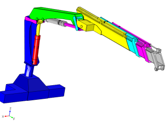
In the Application Libraries window, select Multibody Dynamics Module > Machinery and Robotics > truck_mounted_crane in the tree.
|
|
3
|
Click
|
|
1
|
|
2
|
|
3
|
Click
|
|
4
|
Browse to the model’s Application Libraries folder and double-click the file crane_link_optimization_parameters.txt.
|
|
1
|
|
2
|
|
3
|
|
4
|
|
5
|
|
6
|
|
7
|
|
8
|
|
1
|
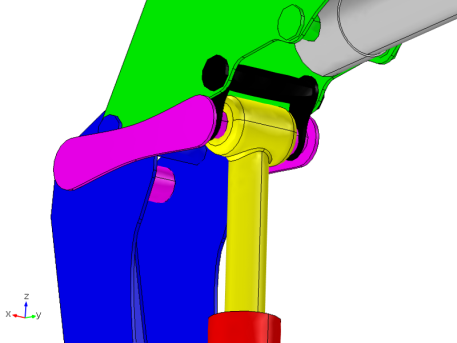
In the Model Builder window, expand the Component 1 (comp1) > Multibody Dynamics (mbd) > Hinge Joints > Hinge Base-Link1 node, then click Hinge Base-Link1.
|
|
2
|
|
3
|
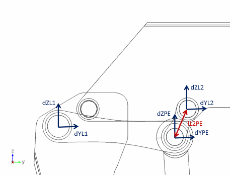
From the list, choose User defined.
|
|
4
|
|
1
|
|
2
|
|
3
|
From the list, choose User defined.
|
|
4
|
|
1
|
In the Model Builder window, expand the Component 1 (comp1) > Multibody Dynamics (mbd) > Slot Joints node, then click Slot Link1-Link2.
|
|
2
|
|
3
|
From the list, choose User defined.
|
|
4
|
|
1
|
|
2
|
|
3
|
From the list, choose User defined.
|
|
4
|
|
1
|
|
2
|
|
1
|
|
2
|
|
5
|
Click
|
|
6
|
|
1
|
In the Model Builder window, expand the Study 1 > Solver Configurations > Solution 1 (sol1) > Dependent Variables 1 node, then click comp1.mbd_rd_rot.
|
|
2
|
|
3
|
|
4
|
|
5
|
|
6
|
|
7
|
|
8
|
|
9
|
|
10
|
|
11
|
|
12
|
|
1
|
|
2
|
|
4
|
Click
|
|
1
|
|
2
|
|
3
|
|
4
|
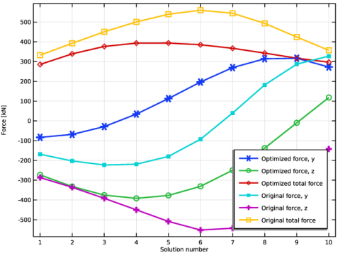
Locate the y-Axis Data section. In the table, enter the following settings:
|
|
1
|
|
2
|
Go to the Add Study window.
|
|
3
|
|
4
|
Click the Add Study button in the window toolbar.
|
|
5
|
|
1
|
|
2
|
|
3
|
|
4
|
|
5
|
|
6
|
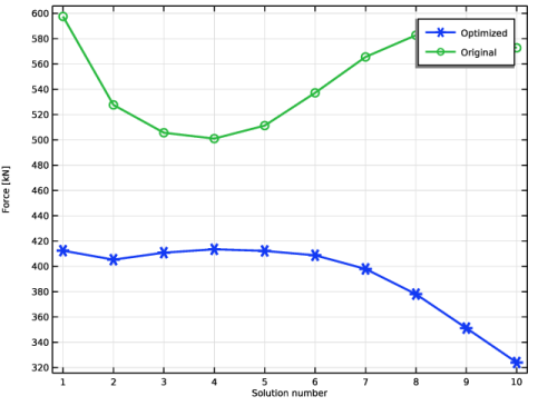
Locate the Objective Function section. In the table, enter the following settings:
|
|
7
|
|
8
|
|
9
|
Browse to the model’s Application Libraries folder and double-click the file crane_link_optimization_ctrlvars.txt.
|
|
10
|
Locate the Constraints section. In the table, enter the following settings:
|
|
11
|
|
13
|
|
14
|
|
15
|
|
16
|
|
1
|
In the Model Builder window, expand the Study 2: Optimization > Solver Configurations > Solution 2 (sol2) > Dependent Variables 1 node, then click Rigid Material Rotations (comp1.mbd_rd_rot).
|
|
2
|
|
3
|
|
4
|
|
5
|
|
6
|
|
7
|
|
8
|
|
9
|
|
10
|
|
1
|
|
2
|
|
3
|
|
1
|
|
2
|
|
3
|
|
1
|
|
2
|
|
4
|
Click
|
|
1
|
|
2
|
|
3
|
|
4
|
Locate the y-Axis Data section. In the table, enter the following settings:
|
|
1
|
|
2
|
|
1
|
|
2
|
|
3
|