PDF

Andrew’s Squeezing Mechanism
Introduction
This model simulates the dynamic behavior of Andrew’s squeezing mechanism. This is a benchmark problem for testing the numerical algorithms in the area of multibody dynamics. It requires small time steps due to a very short time scale of the problem.
The data for this model is taken from Ref. 1. The results of the analysis are compared with the results given in the reference.
Model Definition
The geometry of the Andrew’s mechanism is shown in Figure 1. The geometry consists of seven links interconnected by ten hinge joints. This mechanism is also known as the seven body mechanism.
Figure 1: Model geometry (the center of mass of each link is highlighted).
The links of the mechanism are assumed to be rigid bodies. The mechanism is fixed at four points: O, A, B, and C. The center of mass of each link is shown in Figure 1, and the mass and moment of inertia of each link about its center of mass are given in the Table 1.
The initial values of the angles in the mechanism are given in Table 2. The details about these angles can be obtained in Ref. 2.
Gravity is neglected, and the mechanism is initially at rest. A spring of stiffness c0 = 4530 N/m is attached between point C and point D with an initial length of l0 = 0.07785 m. A moment M0 = 0.033 Nm is prescribed on the right crank, link 1.
Results and Discussion
The computed results are compared with the solution presented in Ref. 1. The computed results are in a very good agreement with the results given in the reference. Figure 2 shows the displacement of the mechanism at t = 0.028 s.
Figure 2: Motion of linkages in Andrew’s mechanism at a particular instant.
Figure 3 displays the time variation of the angles between different links in the Andrew’s mechanism. The computed angles are the function of relative rotations on the hinge joints. The computed angles, shown with solid lines, are in very good agreement with the results given in Ref. 1.
Figure 3: Comparison of time variation of angles in Andrew’s mechanism with Ref. 1. The results obtained in COMSOL are shown with solid lines.
Notes About the COMSOL Implementation
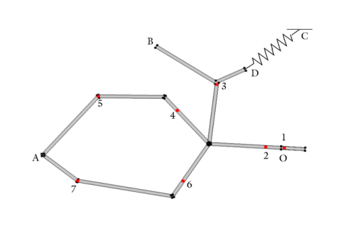
In this model, linkages are modeled as rigid elements using the Rigid Material node as we are only interested in the kinematics of the mechanism. Linkages can be modeled as flexible elements using the Linear Elastic Material node if the stresses and deformations in the linkages are also of interest.
The Mass and Moment of Inertia subnode of the Rigid Material is used to enter the inertia properties given at a certain point.
A Joint node can establish a connection between a Rigid Material or an Attachment node with the ground (Fixed). This helps in avoiding extra geometry components.
The Spring-Damper node is used to connect points C and D with an elastic spring.
The connections set up in the model can be reviewed in the Joints Summary section at the physics interface node.
The net degrees of freedom of this system can be seen in the Rigid Body DOF Summary section at the physics interface node.
References
1. J. Cuadrado, J. Cardenal, and E. Bayo, “Modeling and Solution Methods for Efficient Real-Time Simulation of Multibody Dynamics,” Multibody System Dynamics, vol. 1, pp. 259–280, 1997.
2. W. Schiehlen, Multibody Systems Handbook, Springer-Verlag Berlin Heidelberg, 1990.
Application Library path: Multibody_Dynamics_Module/Verification_Examples/andrews_mechanism
Modeling Instructions
From the File menu, choose New.
New
In the New window, click  Model Wizard.
Model Wizard
1
In the Model Wizard window, click  2D.
2
In the Select Physics tree, select Structural Mechanics > Multibody Dynamics (mbd).
3
Click Add.
4
Click  Study.
5
In the Select Study tree, select General Studies > Time Dependent.
6
Geometry 1
Import 1 (imp1)
1
In the Home toolbar, click  Import.
2
In the Settings window for Import, locate the Source section.
3
Click  Browse.
4
5
Click  Import.
6
Click the  Zoom Extents button in the Graphics toolbar.
Form Union (fin)
1
In the Model Builder window, under Component 1 (comp1) > Geometry 1 click Form Union (fin).
2
In the Settings window for Form Union/Assembly, locate the Form Union/Assembly section.
3
From the Action list, choose Form an assembly.
4
In the Home toolbar, click  Build All.
Global Definitions
Import the inertia properties of all the linkages.
Parameters 1
1
In the Model Builder window, under Global Definitions click Parameters 1.
2
In the Settings window for Parameters, locate the Parameters section.
3
Click  Load from File.
4
Multibody Dynamics (mbd)
Rigid Material 1
1
In the Physics toolbar, click  Domains and choose Rigid Material.
2
Set the density of the selected rigid domain to zero. Use a Mass and Moment of Inertia subnode instead to specify the mass, moment of inertia, and center of mass of the domain.
3
In the Settings window for Rigid Material, locate the Density section.
4
From the ρ list, choose User defined.
Mass and Moment of Inertia 1
1
In the Physics toolbar, click  Attributes and choose Mass and Moment of Inertia.
2
In the Settings window for Mass and Moment of Inertia, locate the Center of Mass section.
3
From the list, choose Centroid of selected entities.
4
From the Entity level list, choose Point.
5
Locate the Mass and Moment of Inertia section. In the m text field, type m1.
6
In the Iz text field, type I1.
Center of Mass: Point 1
1
In the Model Builder window, click Center of Mass: Point 1.
2
Rigid Materials
Similarly, create other rigid domains by duplicating Rigid Material 1 and resetting the inputs using the information given in the table below:
Apply the moment on the crank using an Applied Moment subnode of the rigid material.
Rigid Material 1
In the Model Builder window, under Component 1 (comp1) > Multibody Dynamics (mbd) click Rigid Material 1.
Applied Moment 1
1
In the Physics toolbar, click  Attributes and choose Applied Moment.
2
In the Settings window for Applied Moment, locate the Applied Moment section.
3
In the Mz text field, type M0.
Rigid Material 1, Rigid Material 2, Rigid Material 3, Rigid Material 4, Rigid Material 5, Rigid Material 6, Rigid Material 7
1
In the Model Builder window, under Component 1 (comp1) > Multibody Dynamics (mbd), Ctrl-click to select Rigid Material 1, Rigid Material 2, Rigid Material 3, Rigid Material 4, Rigid Material 5, Rigid Material 6, and Rigid Material 7.
2
Rigid Materials
In the Settings window for Group, type Rigid Materials in the Label text field.
Model the spring connection using a Spring-Damper node.
Spring–Damper 1
1
In the Physics toolbar, click  Global and choose Spring–Damper.
2
In the Settings window for Spring–Damper, locate the Attachment Selection section.
3
From the Source list, choose Fixed.
4
Specify the Xs vector as
5
From the Destination list, choose Rigid Material 3.
6
From the Connection point list, choose Centroid of selected entities.
Destination Point: Boundary 1
1
In the Model Builder window, click Destination Point: Boundary 1.
2
Spring–Damper 1
1
In the Model Builder window, click Spring–Damper 1.
2
In the Settings window for Spring–Damper, locate the Spring section.
3
In the k text field, type c0.
4
Click to expand the Free Length section. From the list, choose Specify free length.
5
In the lf text field, type l0.
Hinge Joint 1
1
In the Physics toolbar, click  Global and choose Hinge Joint.
2
In the Settings window for Hinge Joint, locate the Attachment Selection section.
3
From the Source list, choose Fixed.
4
From the Destination list, choose Rigid Material 1.
5
Locate the Center of Joint section. From the Entity level list, choose Point.
Center of Joint: Point 1
1
In the Model Builder window, click Center of Joint: Point 1.
2
Hinge Joints
Create more joints by duplicating Hinge Joint 1 and resetting the inputs using the information given in the table below:
Hinge Joint 1, Hinge Joint 10, Hinge Joint 2, Hinge Joint 3, Hinge Joint 4, Hinge Joint 5, Hinge Joint 6, Hinge Joint 7, Hinge Joint 8, Hinge Joint 9
1
In the Model Builder window, under Component 1 (comp1) > Multibody Dynamics (mbd), Ctrl-click to select Hinge Joint 1, Hinge Joint 2, Hinge Joint 3, Hinge Joint 4, Hinge Joint 5, Hinge Joint 6, Hinge Joint 7, Hinge Joint 8, Hinge Joint 9, and Hinge Joint 10.
2
Hinge Joints
In the Settings window for Group, type Hinge Joints in the Label text field.
Definitions
Create the following variables for use in the postprocessing.
Some of the angles of the mechanism are modified using the modulus operator in order to obtain the representation used in Ref. 1.
Variables 1
1
In the Definitions toolbar, click  Local Variables.
2
In the Settings window for Variables, locate the Variables section.
3
Study 1
Step 1: Time Dependent
1
In the Model Builder window, under Study 1 click Step 1: Time Dependent.
2
In the Settings window for Time Dependent, locate the Study Settings section.
3
In the Output times text field, type range(0,1e-4,0.03).
4
In the Study toolbar, click  Compute.
Results
Displacement (mbd)
The two default plots show the displacement and velocity profile of the Andrew’s mechanism. The first default plot is shown in Figure 2.
1
In the Settings window for 2D Plot Group, locate the Plot Settings section.
2
From the Frame list, choose Material  (X, Y, Z).
3
Locate the Data section. From the Time (s) list, choose 0.028.
4
Click the  Zoom Extents button in the Graphics toolbar.
5
In the Displacement (mbd) toolbar, click  Plot.
Import the following tables, containing the results obtained in Ref. 1, for comparison.
beta
1
In the Results toolbar, click  Table.
2
In the Settings window for Table, type beta in the Label text field.
3
Locate the Data section. Click  Import.
4
theta
1
In the Results toolbar, click  Table.
2
In the Settings window for Table, type theta in the Label text field.
3
Locate the Data section. Click  Import.
4
gamma
1
In the Results toolbar, click  Table.
2
In the Settings window for Table, type gamma in the Label text field.
3
Locate the Data section. Click  Import.
4
delta
1
In the Results toolbar, click  Table.
2
In the Settings window for Table, type delta in the Label text field.
3
Locate the Data section. Click  Import.
4
phi
1
In the Results toolbar, click  Table.
2
In the Settings window for Table, type phi in the Label text field.
3
Locate the Data section. Click  Import.
4
omega
1
In the Results toolbar, click  Table.
2
In the Settings window for Table, type omega in the Label text field.
3
Locate the Data section. Click  Import.
4
Use the following instructions to plot the time variation of the angles in the mechanism shown in Figure 3.
Angles
1
In the Results toolbar, click  1D Plot Group.
2
In the Settings window for 1D Plot Group, type Angles in the Label text field.
Global 1
1
Right-click Angles and choose Global.
2
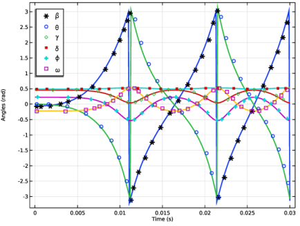
In the Settings window for Global, click Replace Expression in the upper-right corner of the y-Axis Data section. From the menu, choose Component 1 (comp1) > Definitions > Variables > beta - beta - rad.
3
Click Add Expression in the upper-right corner of the y-Axis Data section. From the menu, choose Component 1 (comp1) > Definitions > Variables > theta - theta - rad.
4
Click Add Expression in the upper-right corner of the y-Axis Data section. From the menu, choose Component 1 (comp1) > Definitions > Variables > gamma - gamma - rad.
5
Click Add Expression in the upper-right corner of the y-Axis Data section. From the menu, choose Component 1 (comp1) > Definitions > Variables > delta - delta - rad.
6
Click Add Expression in the upper-right corner of the y-Axis Data section. From the menu, choose Component 1 (comp1) > Definitions > Variables > phi - phi - rad.
7
Click Add Expression in the upper-right corner of the y-Axis Data section. From the menu, choose Component 1 (comp1) > Definitions > Variables > omega - omega - rad.
8
Click to expand the Coloring and Style section. From the Width list, choose 2.
9
Click to expand the Legends section. Clear the Show legends checkbox.
Table Graph 1
1
In the Model Builder window, right-click Angles and choose Table Graph.
2
In the Settings window for Table Graph, locate the Coloring and Style section.
3
Find the Line markers subsection. From the Marker list, choose Cycle.
4
Find the Line style subsection. From the Line list, choose None.
5
Click to expand the Legends section. Select the Show legends checkbox.
6
From the Legends list, choose Manual.
7
Table Graph 2
1
Right-click Table Graph 1 and choose Duplicate.
2
In the Settings window for Table Graph, locate the Data section.
3
From the Table list, choose theta.
4
Locate the Legends section. In the table, enter the following settings:
Table Graph 3
1
Right-click Table Graph 2 and choose Duplicate.
2
In the Settings window for Table Graph, locate the Data section.
3
From the Table list, choose gamma.
4
Locate the Legends section. In the table, enter the following settings:
Table Graph 4
1
Right-click Table Graph 3 and choose Duplicate.
2
In the Settings window for Table Graph, locate the Data section.
3
From the Table list, choose delta.
4
Locate the Legends section. In the table, enter the following settings:
Table Graph 5
1
Right-click Table Graph 4 and choose Duplicate.
2
In the Settings window for Table Graph, locate the Data section.
3
From the Table list, choose phi.
4
Locate the Legends section. In the table, enter the following settings:
Table Graph 6
1
Right-click Table Graph 5 and choose Duplicate.
2
In the Settings window for Table Graph, locate the Data section.
3
From the Table list, choose omega.
4
Locate the Legends section. In the table, enter the following settings:
Angles
1
In the Model Builder window, click Angles.
2
In the Settings window for 1D Plot Group, locate the Legend section.
3
From the Position list, choose Upper left.
4
Click to expand the Title section. From the Title type list, choose None.
5
Locate the Plot Settings section.
6
Select the x-axis label checkbox. In the associated text field, type Time (s).
7
Select the y-axis label checkbox. In the associated text field, type Angles (rad).
8
In the Angles toolbar, click  Plot.
Finally, to generate an animation of Andrew’s mechanism, follow these instructions:
Animation 1
1
In the Results toolbar, click  Animation and choose Player.
2
In the Settings window for Animation, locate the Frames section.
3
In the Number of frames text field, type 100.