PDF

Pacemaker Electrode
Introduction
This example illustrates the use of COMSOL Multiphysics for modeling of ionic current distribution problems in electrolytes, in this case in human tissue. The problem is exemplified on a pacemaker electrode, but it can be applied in electrochemical cells like fuel cells, batteries, corrosion protection, or any other process where ionic conduction takes place in the absence of concentration gradients.
By using the LiveLink interface for Solid Edge you can study the influence of the design of the electrode on the current distribution. The model demonstrates how to synchronize the geometry between Solid Edge and COMSOL Multiphysics while updating dimensional parameters, and how to perform an automatic parametric sweep.
The modeled device is a pacemaker electrode that is placed inside the heart and helps the patient’s heart to keep a normal rhythm. The device is referred to as an electrode, but it actually consists of two electrodes: a cathode and an anode.
Figure 1 shows a schematic drawing of two pair of electrodes placed inside the heart. The electrodes are supplied with current from the pulse generator unit, which is also implanted in the patient.
Figure 1: Schematic drawing of the heart with two pairs of pacemaker electrodes.
This example deals with the current and potential distribution around one pair of electrodes.
Model Definition
The model domain consists of the blood and tissue surrounding the electrode pair. The actual electrodes and the electrode support are boundaries to the modeled domain. Figure 2 shows the electrode in a darker shade, while the surrounding modeling domain is shown in a lighter shade.
Figure 2: Modeling domain and boundaries.
The working electrode consists of a hemisphere placed on the tip of the supporting cylindrical structure. The counter electrode is placed in the “waist” of this structure. All other surfaces of the supporting structure are insulated. The outer boundaries are placed far enough from the electrode to give a small impact on the current and potential distribution.
In COMSOL Multiphysics, use the Electric Currents interface for the analysis of the electrode. This physics interface is useful for modeling conductive materials where a current flows due to an applied electric field.
Domain Equations
The current in the domain is controlled by the continuity equation, which follows from Maxwell’s equations:
where σ is the conductivity of the human heart. This equation uses the following relations between the electric potential and the fields.
Boundary Conditions
Ground potential boundary conditions are applied on the thinner waist of the electrode. The tip of the electrode has a fixed potential of 1 V. All other boundaries are electrically insulated.
Results and Discussion
This simulation gives the potential distribution on the electrode surface and streamlines of the current distribution inside the human heart; see Figure 3.
Figure 3: The plot shows the electrostatic potential distributed on the surface of the electrode. The total current density is shown as streamlines.
As expected, the current density is highest at the small hemisphere, which is the one that causes the excitation of the heart. The current density is fairly uniform on the working electrode. The counter electrode is larger and there are also larger variations in current density on its surface. Mainly, the current is lower with the distance from the working electrode. The model shows that the anchoring arms of the device have little influence on the current density distribution.
Moving the location of the counter electrode closer to the anchoring arms on the device have little influence on the current distribution. The position of the counter electrode affects the electric resistance of the pacemaker electrode, which is important when designing the electrical circuit, in which the pacemaker electrode is included; see Figure 4, which shows a plot of the electric resistance of the pacemaker electrode for different values of the distance between counter electrode and working electrode.
Figure 4: The plot shows the electric resistance of the pacemaker electrode in relation to the distance between the counter electrode and the working electrode.
Notes About the COMSOL Implementation
The pacemaker electrode geometry you are using in this model comes from a Solid Edge part. The LiveLink interface transfers the geometry from Solid Edge to COMSOL Multiphysics. Using the interface you are also able to update the dimension of the electrode in the Solid Edge file. In order for this to work you need to have both programs running during modeling, and you need to make sure that the file of the pacemaker electrode is the active file in Solid Edge.
Application Library path: LiveLink_for_Solid_Edge/Tutorials,_LiveLink_Interface/pacemaker_electrode_llse
Modeling Instructions
1
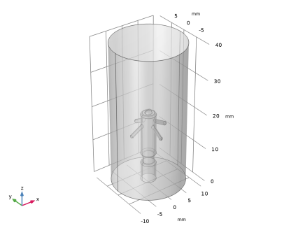
In Solid Edge open the file pacemaker_electrode.par located in the model’s Application Library folder.
2
COMSOL Desktop
From the File menu, choose New.
New
In the New window, click  Model Wizard.
Model Wizard
1
In the Model Wizard window, click  3D.
2
In the Select Physics tree, select AC/DC > Electric Fields and Currents > Electric Currents (ec).
3
Click Add.
4
Click  Study.
5
In the Select Study tree, select General Studies > Stationary.
6
Geometry 1
Make sure that the CAD Import Module kernel is used.
1
In the Model Builder window, under Component 1 (comp1) click Geometry 1.
2
In the Settings window for Geometry, locate the Advanced section.
3
From the Geometry representation list, choose CAD kernel.
LiveLink for Solid Edge 1 (cad1)
1
In the Home toolbar, click  LiveLink and choose LiveLink for Solid Edge.
2
In the Settings window for LiveLink for Solid Edge, locate the Synchronize section.
3
Click Synchronize.
After a few moments the geometry of the pacemaker electrode appears in the Graphics window.
4
Click the  Transparency button in the Graphics toolbar.
5
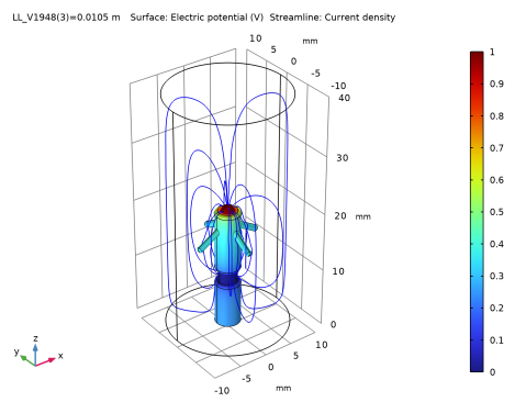
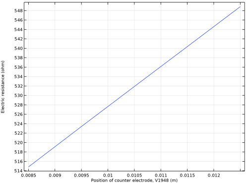
Click to expand the Parameters in CAD Package section. The dimensional parameter for the position of the counter electrode, V1948 in the Solid Edge file, has been linked to COMSOL Multiphysics and is therefore synchronized with the geometry. To manage linked parameters, you can click Parameter Selection on the COMSOL Multiphysics tab in Solid Edge. The global parameter, LL_V1948, is automatically generated in the COMSOL Multiphysics model during synchronization to enable parametric sweeps and optimization of the geometry.
6
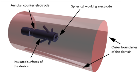
Click to expand the Boundary Selections section. The selections listed here are user defined selections saved in the Solid Edge file. In Solid Edge, you can set up selections using the Selections button on the COMSOL Multiphysics tab.
Global Definitions
Parameters 1
The table already contains the automatically generated global parameter that is linked to the dimension inside Solid Edge. It is possible to edit the value of the parameter here, and then synchronize, to modify the geometry. But in this tutorial we will use the parametric solver to automatically solve the model for a range of parameter values.
Continue with loading additional parameters for setting up the physics.
1
In the Model Builder window, under Global Definitions click Parameters 1.
2
In the Settings window for Parameters, locate the Parameters section.
3
Click  Load from File.
4
Definitions
Integration 1 (intop1)
The integration operator you will set up in the next steps is used to evaluate the electric resistance of the pacemaker electrode.
1
In the Definitions toolbar, click  Nonlocal Couplings and choose Integration.
2
In the Settings window for Integration, type my_int in the Operator name text field.
3
Locate the Source Selection section. From the Geometric entity level list, choose Boundary.
4
From the Selection list, choose Counter electrode.
5
Locate the Advanced section. From the Method list, choose Summation over nodes.
Materials
Heart Tissue
1
In the Model Builder window, under Component 1 (comp1) right-click Materials and choose Blank Material.
2
In the Settings window for Material, locate the Material Contents section.
3
4
Right-click Material 1 (mat1) and choose Rename.
5
In the Rename Material dialog, type Heart Tissue in the New label text field.
6
Electric Currents (ec)
Ground 1
1
In the Physics toolbar, click  Boundaries and choose Ground.
2
In the Settings window for Ground, locate the Boundary Selection section.
3
From the Selection list, choose Counter electrode.
Electric Potential 1
1
In the Physics toolbar, click  Boundaries and choose Electric Potential.
2
In the Settings window for Electric Potential, locate the Boundary Selection section.
3
From the Selection list, choose Working electrode.
4
Locate the Electric Potential section. In the V0 text field, type Vtot.
Mesh 1
1
In the Model Builder window, under Component 1 (comp1) click Mesh 1.
2
In the Settings window for Mesh, locate the Physics-Controlled Mesh section.
3
From the Element size list, choose Fine.
4
Click  Build All.
Study 1
In the Study toolbar, click  Compute.
Results
Evaluation Group 1
In the Results toolbar, click  Evaluation Group.
Global Evaluation 1
1
Right-click Evaluation Group 1 and choose Global Evaluation.
2
In the Settings window for Global Evaluation, locate the Expressions section.
3
4
In the Evaluation Group 1 toolbar, click  Evaluate.
3D Plot Group 3
In the Home toolbar, click  Add Plot Group and choose 3D Plot Group.
Surface 1
Right-click 3D Plot Group 3 and choose Surface.
Selection 1
1
In the Model Builder window, right-click Surface 1 and choose Selection.
2
In the Settings window for Selection, locate the Selection section.
3
From the Selection list, choose Pacemaker.
Streamline 1
1
In the Model Builder window, right-click 3D Plot Group 3 and choose Streamline.
2
In the Settings window for Streamline, locate the Streamline Positioning section.
3
From the Positioning list, choose Starting-point controlled.
4
Locate the Coloring and Style section. Find the Point style subsection. From the Color list, choose Blue.
5
In the 3D Plot Group 3 toolbar, click  Plot.
6
Click the  Transparency button in the Graphics toolbar.
You should see a plot similar to the plot in Figure 3.
Study 1
Parametric Sweep
1
In the Study toolbar, click  Parametric Sweep.
2
In the Settings window for Parametric Sweep, locate the Study Settings section.
3
4
Click  Range.
5
In the Range dialog, type 8.5[mm] in the Start text field.
6
In the Step text field, type 1[mm].
7
In the Stop text field, type 12.5[mm].
8
Click Add.
9
In the Study toolbar, click  Compute.
Results
Evaluation Group 1
1
In the Model Builder window, click Evaluation Group 1.
2
In the Settings window for Evaluation Group, locate the Data section.
3
From the Dataset list, choose Study 1/Parametric Solutions 1 (sol2).
4
In the Evaluation Group 1 toolbar, click  Evaluate.
Evaluation Group 1
1
Go to the Evaluation Group 1 window.
2
Click the Table Graph button in the window toolbar.
Results
1D Plot Group 6
1
In the Model Builder window, click 1D Plot Group 6.
2
In the Settings window for 1D Plot Group, locate the Plot Settings section.
3
Select the x-axis label checkbox. In the associated text field, type Position of counter electrode, V1948 (m).
4
Select the y-axis label checkbox. In the associated text field, type Electric resistance (ohm).
5
In the 1D Plot Group 6 toolbar, click  Plot.
You should see a plot similar to the plot in Figure 4.
3D Plot Group 7
1
In the Results toolbar, click  3D Plot Group.
2
In the Settings window for 3D Plot Group, locate the Data section.
3
From the Dataset list, choose Study 1/Parametric Solutions 1 (sol2).
4
From the Parameter value (LL_V1948 (m)) list, choose 0.0105.
Surface 1
Right-click 3D Plot Group 7 and choose Surface.
Selection 1
1
In the Model Builder window, right-click Surface 1 and choose Selection.
2
In the Settings window for Selection, locate the Selection section.
3
From the Selection list, choose Pacemaker.
Streamline 1
1
In the Model Builder window, right-click 3D Plot Group 7 and choose Streamline.
2
In the Settings window for Streamline, locate the Streamline Positioning section.
3
From the Positioning list, choose Starting-point controlled.
4
Locate the Coloring and Style section. Find the Point style subsection. From the Color list, choose Blue.
5
In the 3D Plot Group 7 toolbar, click  Plot.
The plot should now look similar to the one displayed below.