
|
|
|

|
3
|
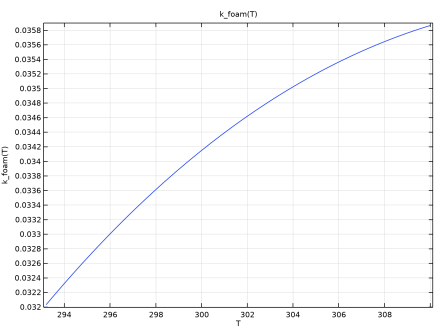
Save the file as k_foam.m.
|
|
5
|
Save the file as k_foam_dT.m.
|
|
7
|
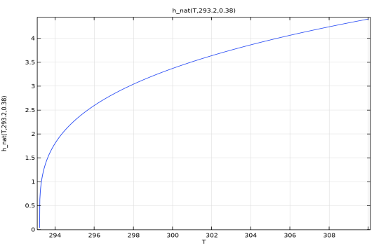
Save the file as h_nat.m.
|
|
9
|
Save the file as h_nat_dT.m.
|
|
1
|
|
2
|
|
3
|
Click Add.
|
|
4
|
Click
|
|
5
|
|
6
|
Click
|
|
1
|
|
2
|
|
1
|
|
2
|
|
4
|
Click to expand the Plot Parameters section. In the table, enter the following settings:
|
|
5
|
Click
|
|
6
|
Locate the Functions section. In the table, enter the following settings:
|
|
7
|
Click
|
|
8
|
Locate the Plot Parameters section. In the table, enter the following settings:
|
|
9
|
Click
|
|
10
|
Click to expand the Derivatives section. In the table, enter the following settings:
|
|
11
|
Locate the Functions section. In the table, enter the following settings:
|
|
1
|
|
2
|
|
3
|
Click
|
|
4
|
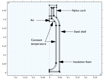
Browse to the model’s Application Libraries folder and double-click the file vacuum_flask_llmatlab.dxf.
|
|
5
|
Click
|
|
1
|
|
2
|
|
3
|
|
1
|
|
2
|
|
1
|
|
2
|
Click
|
|
3
|
|
4
|
Click
|
|
5
|
Click
|
|
1
|
|
3
|
|
5
|
|
6
|
|
7
|
Click OK.
|
|
1
|
|
3
|
|
5
|
|
6
|
|
7
|
Click OK.
|
|
1
|
|
3
|
|
4
|
|
1
|
|
3
|
|
4
|
|
5
|
|
6
|
|
1
|
|
2
|
|
3
|
|
4
|
Click
|
|
1
|
|
2
|
Go to the Result Templates window.
|
|
3
|
|
4
|
Click the Add Result Template button in the window toolbar.
|
|
5
|
|
1
|
|
3
|
|
4
|
|
5
|
|
6
|
|
7
|