|
|
|


|
1
|
|
2
|
In the Select Physics tree, select Heat Transfer > Heat and Moisture Transport > Building Materials.
|
|
3
|
Click Add.
|
|
4
|
Click
|
|
5
|
|
6
|
Click
|
|
1
|
|
2
|
|
1
|
|
2
|
|
1
|
In the Model Builder window, under Component 1 (comp1) right-click Materials and choose Blank Material.
|
|
2
|
|
3
|
In the Model Builder window, expand the Component 1 (comp1) > Materials > Material - Norm 15026 (mat1) node.
|
|
4
|
In the Model Builder window, under Component 1 (comp1) > Materials > Material - Norm 15026 (mat1) click Basic (def).
|
|
5
|
|
6
|
Click
|
|
7
|
|
8
|
|
9
|
Click OK.
|
|
1
|
|
2
|
|
3
|
|
4
|
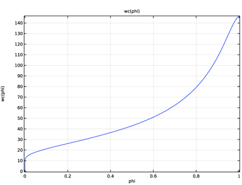
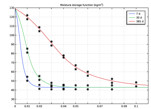
Locate the Definition section. In the Expression text field, type 146/(1+(-8e-8*462*293.15*1000*log(phi))^1.6)^0.375.
|
|
5
|
|
6
|
Click
|
|
1
|
|
2
|
|
3
|
|
4
|
|
5
|
|
6
|
Locate the Plot Parameters section. In the table, enter the following settings:
|
|
7
|
Click
|
|
1
|
|
2
|
|
3
|
|
4
|
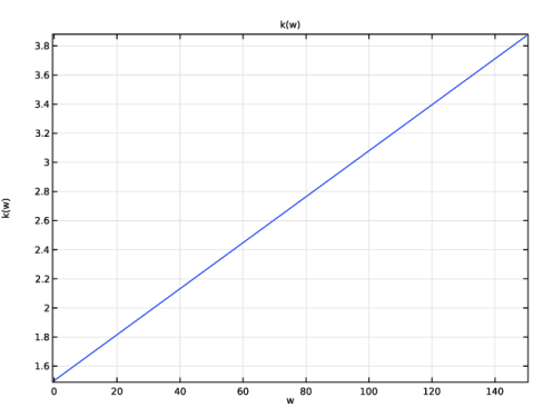
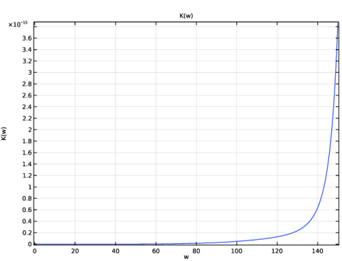
Locate the Definition section. In the Expression text field, type 0.125e8*((146/w)^(1/0.375)-1)^0.625.
|
|
5
|
|
6
|
Locate the Plot Parameters section. In the table, enter the following settings:
|
|
7
|
Click
|
|
1
|
|
2
|
|
3
|
|
4
|
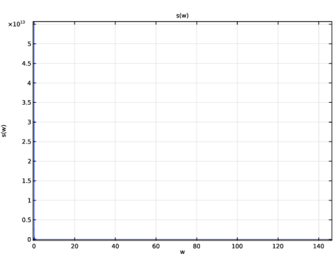
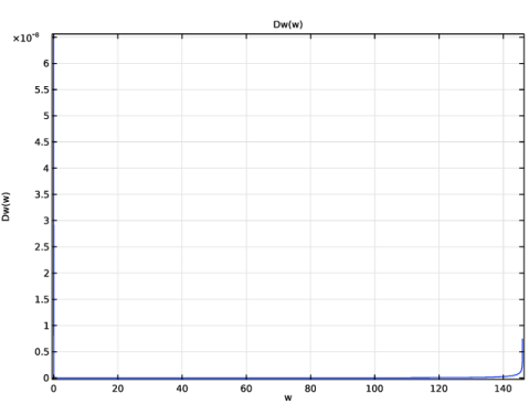
Locate the Definition section. In the Expression text field, type exp(-39.2619+0.0704*(w-146/2)-1.7420e-4*(w-146/2)^2-2.7953e-6*(w-146/2)^3-1.1566e-7*(w-146/2)^4+2.5969e-9*(w-146/2)^5).
|
|
5
|
|
6
|
Locate the Plot Parameters section. In the table, enter the following settings:
|
|
7
|
Click
|
|
1
|
|
2
|
|
3
|
|
4
|
|
5
|
|
6
|
Locate the Plot Parameters section. In the table, enter the following settings:
|
|
7
|
Click
|
|
1
|
|
2
|
|
3
|
|
4
|
Locate the Definition section. In the Expression text field, type (0.01801528/R_const/293.15*26.1e-6/200*(1-w/146)/((1-0.497)*(1-w/146)^2+0.497)).
|
|
5
|
|
6
|
Locate the Plot Parameters section. In the table, enter the following settings:
|
|
1
|
|
2
|
|
1
|
In the Model Builder window, under Component 1 (comp1) > Materials click Material - Norm 15026 (mat1).
|
|
2
|
|
1
|
|
2
|
|
3
|
|
4
|
|
5
|
Select the Cutoff checkbox.
|
|
6
|
|
7
|
Select the Size of transition zone at cutoff checkbox.
|
|
8
|
|
9
|
|
1
|
In the Model Builder window, under Component 1 (comp1) > Heat Transfer in Building Materials (ht) click Initial Values 1.
|
|
2
|
|
3
|
|
1
|
|
3
|
|
4
|
|
1
|
|
3
|
|
4
|
|
1
|
In the Model Builder window, under Component 1 (comp1) > Moisture Transport in Building Materials (mt) click Initial Values 1.
|
|
2
|
|
3
|
|
1
|
|
3
|
|
4
|
|
5
|
|
1
|
|
3
|
|
4
|
|
5
|
|
1
|
|
2
|
|
3
|
|
4
|
|
5
|
|
6
|
Click
|
|
1
|
|
2
|
|
3
|
|
4
|
|
5
|
|
6
|
|
7
|
|
1
|
|
2
|
|
3
|
Click
|
|
4
|
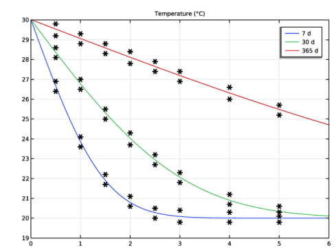
Browse to the model’s Application Libraries folder and double-click the file semi_infinite_wall_temperature.txt.
|
|
1
|
|
2
|
|
3
|
Click
|
|
4
|
Browse to the model’s Application Libraries folder and double-click the file semi_infinite_wall_moisture_storage_function.txt.
|
|
1
|
|
2
|
|
3
|
Select the Manual axis limits checkbox.
|
|
4
|
|
5
|
|
6
|
|
7
|
|
8
|
|
9
|
|
1
|
|
2
|
|
3
|
|
4
|
|
5
|
|
1
|
|
2
|
|
3
|
|
4
|
|
5
|
|
6
|
|
1
|
|
2
|
|
3
|
|
4
|
|
5
|
|
6
|
|
7
|
|
8
|
|
9
|
|
1
|
|
2
|
|
3
|
|
4
|
|
5
|
|
6
|
|
1
|
|
2
|
|
3
|
|
4
|
Locate the Coloring and Style section. Find the Line style subsection. From the Line list, choose None.
|
|
5
|
|
6
|
|
7
|