|
|
|
|
1
|
|
2
|
|
3
|
Click Add.
|
|
4
|
|
5
|
Click Add.
|
|
6
|
Click
|
|
7
|
|
8
|
Click
|
|
1
|
|
2
|
|
1
|
|
2
|
|
3
|
|
1
|
|
2
|
|
3
|
|
4
|
|
5
|
Click
|
|
1
|
|
2
|
|
3
|
|
4
|
|
5
|
|
6
|
Click
|
|
1
|
|
2
|
|
3
|
|
4
|
|
5
|
|
6
|
Click
|
|
1
|
|
2
|
|
3
|
|
4
|
|
5
|
|
6
|
|
7
|
Click
|
|
1
|
|
2
|
|
3
|
|
4
|
|
5
|
|
6
|
|
7
|
Click
|
|
1
|
|
2
|
|
3
|
|
4
|
|
5
|
Click
|
|
1
|
|
2
|
|
3
|
|
4
|
|
5
|
|
6
|
|
1
|
|
2
|
|
3
|
|
1
|
|
3
|
|
4
|
Click
|
|
5
|
|
6
|
Click OK.
|
|
1
|
In the Model Builder window, under Component 1 (comp1) > Heat Transfer in Solids and Fluids (ht) click Fluid 1.
|
|
2
|
|
3
|
|
1
|
|
2
|
Go to the Add Material window.
|
|
3
|
|
4
|
Click the Add to Component button in the window toolbar.
|
|
1
|
|
2
|
|
4
|
Locate the Material Contents section. In the table, enter the following settings:
|
|
1
|
|
2
|
|
4
|
Locate the Material Contents section. In the table, enter the following settings:
|
|
1
|
|
2
|
|
4
|
Locate the Material Contents section. In the table, enter the following settings:
|
|
1
|
Go to the Add Material window.
|
|
2
|
|
3
|
Click the Add to Component button in the window toolbar.
|
|
4
|
|
1
|
|
2
|
|
3
|
Locate the Geometric Entity Selection section. From the Geometric entity level list, choose Boundary.
|
|
5
|
Locate the Material Contents section. In the table, enter the following settings:
|
|
1
|
|
2
|
|
3
|
Locate the Geometric Entity Selection section. From the Geometric entity level list, choose Boundary.
|
|
5
|
Locate the Material Contents section. In the table, enter the following settings:
|
|
1
|
|
3
|
|
4
|
|
1
|
|
3
|
|
4
|
|
1
|
|
1
|
|
3
|
|
4
|
|
1
|
|
3
|
|
4
|
|
1
|
|
3
|
|
4
|
|
1
|
|
1
|
|
1
|
In the Model Builder window, under Component 1 (comp1) > Surface-to-Surface Radiation (rad) click Diffuse Surface 1.
|
|
2
|
|
3
|
|
1
|
|
2
|
Go to the Add Multiphysics window.
|
|
3
|
In the tree, select No Predefined Multiphysics Available for the Selected Physics Interfaces.
|
|
4
|
Find the Select the physics interfaces you want to couple subsection. In the table, clear the Couple checkbox for Laminar Flow (spf).
|
|
5
|
|
6
|
Click the Add to Component button in the window toolbar.
|
|
7
|
|
1
|
|
2
|
|
3
|
Click
|
|
1
|
|
1
|
|
2
|
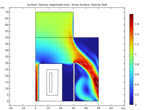
In the Settings window for Arrow Surface, click Replace Expression in the upper-right corner of the Expression section. From the menu, choose Component 1 (comp1) > Laminar Flow > Velocity and pressure > u,w - Velocity field.
|
|
3
|
|
4
|
|
1
|
|
2
|
|
1
|
|
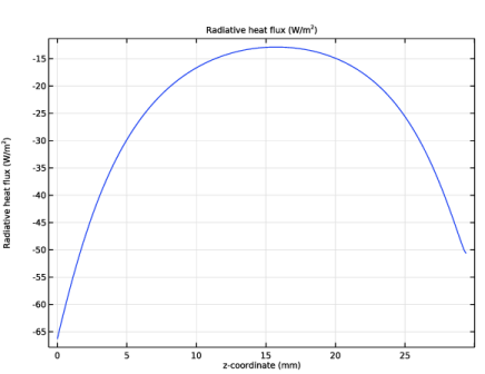
3
|
In the Settings window for Line Graph, click Replace Expression in the upper-right corner of the y-Axis Data section. From the menu, choose Component 1 (comp1) > Surface-to-Surface Radiation > Radiative heat flux > rad.rflux - Radiative heat flux - W/m².
|
|
4
|
Click Replace Expression in the upper-right corner of the x-Axis Data section. From the menu, choose Component 1 (comp1) > Geometry > Coordinate > z - z-coordinate.
|
|
5
|
|
1
|
|
2
|
|
3
|
|
4
|
|
1
|
|
2
|
|
3
|
|
4
|
|
1
|
|
2
|
Go to the Result Templates window.
|
|
3
|
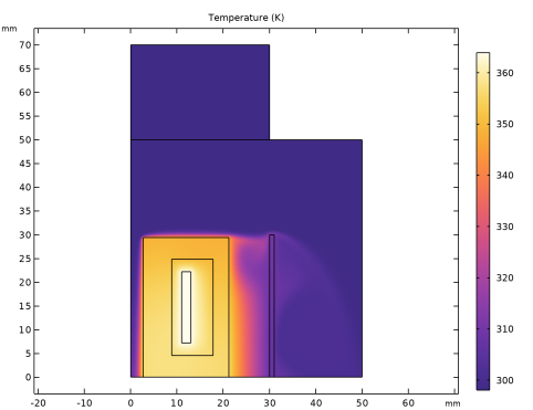
In the tree, select Study 1/Solution 1 (sol1) > Heat Transfer in Solids and Fluids > Temperature (ht).
|
|
4
|
Click the Add Result Template button in the window toolbar.
|
|
5
|
|
1
|
|
2
|
|
1
|
|
2
|
|
1
|
|
2
|
|
3
|
|
4
|
|
5
|
|
6
|