
|
|
|


|
1
|
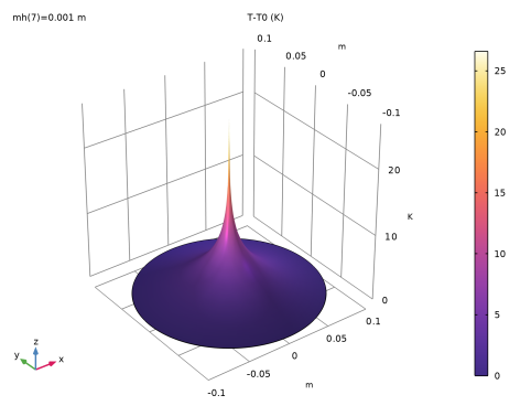
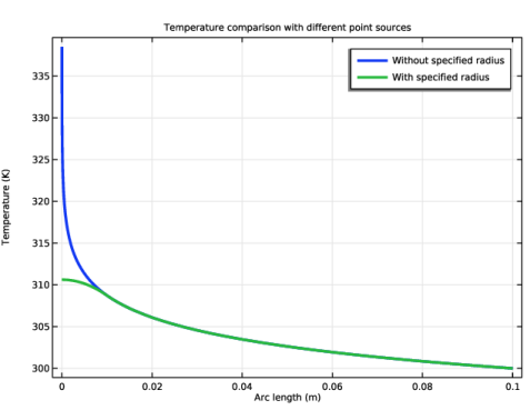
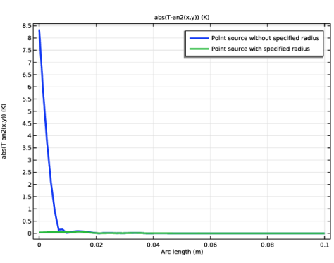
The source support can be defined as a geometrical point. In this case, use the Line Heat Source (2D and 2D axisymmetric), Point Heat Source on Axis (2D axisymmetric) or Point Heat Source (3D) features. This leads to a singularity in the temperature field at the point where the source is applied. Numerically, the finer the mesh, the larger the temperature variation. In general, the two alternatives described below should be considered instead of this option, except for cases where a singular source is needed.
|
|
2
|
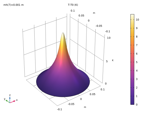
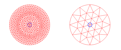
The heat source definition described above can be modified so that COMSOL Multiphysics accounts for the source size without needing a mesh nor a geometry change. In Line Heat Source (2D and 2D axisymmetric), Point Heat Source on Axis (2D axisymmetric) or Point Heat Source (3D) features, select the Specify heat source radius checkbox and set the Heat source radius to Rsource. Then the heat source is automatically distributed over a disk in 2D (a torus in 2D axisymmetric or a sphere in 3D) as illustrated by the blue circle on the right image of Figure 5, even if the mesh elements size is larger than Rsource.
|
|
3
|
If the size of the source is not too small compared to the surrounding geometry details, then a domain representing the heat source can be drawn (see the disk of radius Rsource on the left image of Figure 5) and a Heat Source feature can be defined there. This option can be considered when the increase of the number of mesh elements induced by the geometry change can be afforded.
 |
|
1
|
|
2
|
|
3
|
Click Add.
|
|
4
|
Click
|
|
5
|
|
6
|
Click
|
|
1
|
|
2
|
|
1
|
|
2
|
|
3
|
|
4
|
|
5
|
Locate the Units section. In the table, enter the following settings:
|
|
6
|
|
7
|
Locate the Plot Parameters section. In the table, enter the following settings:
|
|
8
|
Click
|
|
1
|
|
2
|
|
3
|
In the Expression text field, type if(sqrt(x^2+y^2)>R_source, (-1/(2*pi*k_cork)*log(sqrt(x^2+y^2)/R_disk) + T0), (1/(2*pi*k_cork)*(-(x^2+y^2)/(2*R_source^2)+0.5-log(R_source/R_disk)) + T0)).
|
|
4
|
|
5
|
Locate the Plot Parameters section. In the table, enter the following settings:
|
|
6
|
Locate the Units section. In the table, enter the following settings:
|
|
7
|
|
8
|
Click
|
|
1
|
|
2
|
|
3
|
|
1
|
|
2
|
|
1
|
|
2
|
|
3
|
Locate the Material Contents section. In the table, enter the following settings:
|
|
1
|
|
2
|
|
3
|
|
4
|
|
1
|
|
3
|
|
4
|
|
5
|
|
1
|
|
2
|
|
3
|
From the list, choose User-controlled mesh.
|
|
1
|
|
2
|
|
3
|
|
1
|
|
2
|
|
3
|
|
5
|
|
6
|
Click the Custom button.
|
|
7
|
Locate the Element Size Parameters section.
|
|
8
|
|
9
|
Click
|
|
1
|
|
2
|
|
3
|
|
1
|
|
2
|
|
3
|
|
1
|
|
2
|
|
1
|
|
2
|
|
3
|
Click
|
|
4
|
Select mh from the list.
|
|
5
|
Click
|
|
6
|
|
7
|
|
8
|
|
9
|
|
10
|
Click Replace.
|
|
11
|
|
1
|
|
2
|
|
3
|
|
1
|
|
2
|
|
3
|
|
1
|
|
2
|
Click
|
|
3
|
|
1
|
|
2
|
In the Settings window for 1D Plot Group, type L2 Error from Analytical Solution - Study 1 in the Label text field.
|
|
3
|
Locate the Data section. From the Dataset list, choose Study 1: Point Source/Parametric Solutions 1 (sol2).
|
|
1
|
|
2
|
|
3
|
|
4
|
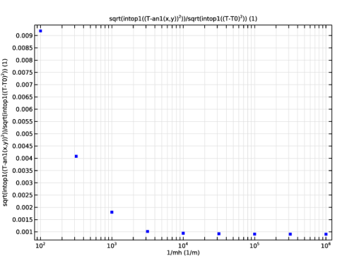
Locate the y-Axis Data section. In the Expression text field, type sqrt(intop1((T-an1(x,y))^2))/sqrt(intop1((T-T0)^2)).
|
|
5
|
|
6
|
|
7
|
|
8
|
|
9
|
|
10
|
|
1
|
|
2
|
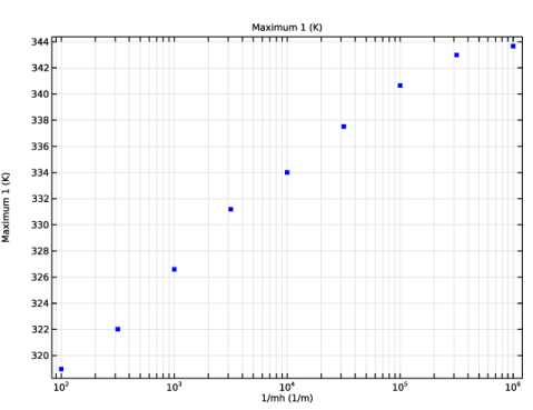
In the Settings window for 1D Plot Group, type Maximum Temperature - Study 1 in the Label text field.
|
|
3
|
Locate the Data section. From the Dataset list, choose Study 1: Point Source/Parametric Solutions 1 (sol2).
|
|
1
|
|
2
|
|
3
|
|
4
|
|
5
|
|
6
|
|
7
|
|
8
|
|
9
|
|
10
|
|
1
|
|
3
|
|
4
|
|
5
|
|
6
|
|
7
|
|
1
|
|
2
|
|
3
|
Select the Modify model configuration for study step checkbox.
|
|
4
|
|
5
|
Right-click and choose Disable.
|
|
1
|
|
2
|
Go to the Add Study window.
|
|
3
|
|
4
|
Click the Add Study button in the window toolbar.
|
|
5
|
|
1
|
|
2
|
Select the Modify model configuration for study step checkbox.
|
|
3
|
|
4
|
Right-click and choose Disable.
|
|
5
|
|
6
|
|
1
|
|
2
|
|
3
|
Click
|
|
4
|
Select mh from the list.
|
|
5
|
Click
|
|
6
|
|
7
|
|
8
|
|
9
|
|
10
|
Click Replace.
|
|
11
|
|
1
|
|
2
|
|
3
|
|
1
|
|
2
|
|
3
|
|
1
|
|
2
|
Click
|
|
3
|
|
1
|
|
2
|
|
3
|
|
4
|
|
5
|
Click
|
|
1
|
|
2
|
In the Settings window for 1D Plot Group, type Analytical Solutions, Point Source with/without Radius in the Label text field.
|
|
3
|
|
4
|
|
5
|
|
6
|
|
7
|
Locate the Plot Settings section.
|
|
8
|
|
1
|
|
2
|
|
3
|
|
4
|
|
5
|
|
6
|
|
1
|
|
2
|
|
3
|
|
4
|
|
5
|
|
6
|
|
7
|
|
9
|
|
1
|
|
2
|
In the Settings window for 1D Plot Group, type Temperature vs. Radius - Study 2 in the Label text field.
|
|
3
|
|
4
|
|
1
|
|
2
|
|
3
|
|
4
|
|
5
|
|
6
|
|
7
|
|
8
|
|
1
|
|
2
|
|
3
|
|
4
|
|
5
|
|
6
|
|
8
|
|
1
|
|
2
|
In the Settings window for 1D Plot Group, type L2 Error from Analytical Solution - Study 2 in the Label text field.
|
|
3
|
Locate the Data section. From the Dataset list, choose Study 2: Point Source with Radius/Parametric Solutions 2 (sol13).
|
|
1
|
|
2
|
|
3
|
|
4
|
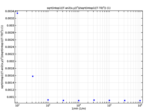
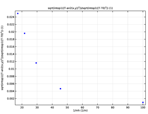
Locate the y-Axis Data section. In the Expression text field, type sqrt(intop1((T-an2(x,y))^2))/sqrt(intop1((T-T0)^2)).
|
|
5
|
|
6
|
|
7
|
|
8
|
|
9
|
|
10
|
|
1
|
|
2
|
|
3
|
|
4
|
|
5
|
Click
|
|
1
|
|
2
|
In the Settings window for 1D Plot Group, type L1 Error from Analytical Solutions - Study 1 and Study 2 in the Label text field.
|
|
3
|
|
4
|
|
1
|
|
2
|
|
3
|
|
4
|
|
5
|
|
6
|
|
1
|
|
2
|
|
3
|
|
4
|
|
5
|
|
6
|
|
7
|
|
8
|
|
9
|
|
11
|
|
1
|
|
2
|
|
3
|
From the list, choose User-controlled mesh.
|
|
1
|
|
2
|
|
3
|
Click the Custom button.
|
|
4
|
|
5
|
|
6
|
Click
|
|
1
|
|
2
|
Go to the Add Study window.
|
|
3
|
|
4
|
Click the Add Study button in the window toolbar.
|
|
5
|
|
1
|
|
2
|
Select the Modify model configuration for study step checkbox.
|
|
3
|
|
4
|
Right-click and choose Disable.
|
|
5
|
|
6
|
In the Settings window for Study, type Study 3: Point Source with Radius, Coarse Mesh in the Label text field.
|
|
1
|
|
2
|
|
3
|
Click
|
|
4
|
Select mh from the list.
|
|
5
|
Click
|
|
6
|
|
7
|
|
8
|
|
9
|
Click Replace.
|
|
10
|
|
1
|
|
1
|
|
2
|
|
3
|
|
4
|
Select the Wireframe checkbox.
|
|
1
|
|
2
|
|
3
|
|
4
|
|
5
|
|
6
|
|
7
|
|
8
|
|
9
|
Clear the Color legend checkbox.
|
|
10
|
|
11
|
|
1
|
|
2
|
|
3
|
|
4
|
|
1
|
|
2
|
In the Settings window for 1D Plot Group, type L2 Error from Analytical Solution - Study 3 in the Label text field.
|
|
3
|
Locate the Data section. From the Dataset list, choose Study 3: Point Source with Radius, Coarse Mesh/Parametric Solutions 3 (sol24).
|
|
1
|
|
2
|
|
3
|
|
4
|
Locate the y-Axis Data section. In the Expression text field, type sqrt(intop1((T-an2(x,y))^2))/sqrt(intop1((T-T0)^2)).
|
|
5
|
|
6
|
|
7
|
|
8
|
|
9
|
|
1
|
|
2
|
|
3
|
|
4
|
|
5
|
Click Import.
|
|
1
|
|
2
|
|
3
|
|
4
|
Click
|
|
1
|
|
2
|
Go to the Add Physics window.
|
|
3
|
|
4
|
Find the Physics interfaces in study subsection. In the table, clear the Solve checkboxes for Study 1: Point Source, Study 2: Point Source with Radius, and Study 3: Point Source with Radius, Coarse Mesh.
|
|
5
|
Click the Add to Component 2 button in the window toolbar.
|
|
6
|
|
1
|
|
3
|
|
4
|
|
1
|
|
3
|
|
4
|
|
5
|
|
1
|
|
2
|
|
3
|
Locate the Material Contents section. In the table, enter the following settings:
|
|
1
|
|
2
|
Go to the Add Study window.
|
|
3
|
|
4
|
Find the Physics interfaces in study subsection. In the table, clear the Solve checkbox for Heat Transfer in Solids (ht).
|
|
5
|
Click the Add Study button in the window toolbar.
|
|
6
|
|
1
|
|
2
|
|
1
|
|
2
|
|
3
|
|
4
|
|
5
|
Click
|
|
1
|
|
2
|
In the Settings window for 1D Plot Group, type Temperature vs. Radius - Study 4 in the Label text field.
|
|
3
|
|
1
|
|
2
|
|
3
|
|
4
|
|
5
|
|
6
|
|
7
|
|
8
|
|
1
|
|
2
|
|
3
|
|
4
|
|
5
|
|
6
|
|
8
|