|
|
|
|
1
|
|
2
|
|
3
|
Click Add.
|
|
4
|
|
5
|
Click Add.
|
|
6
|
Click
|
|
7
|
|
8
|
Click
|
|
1
|
|
2
|
|
3
|
|
1
|
|
2
|
Browse to the model’s Application Libraries folder and double-click the file light_bulb_geom_sequence.mph.
|
|
3
|
|
4
|
|
1
|
|
2
|
|
1
|
|
2
|
Go to the Add Material window.
|
|
3
|
In the tree, select Material Library > Elements > Tungsten > Tungsten [solid] > Tungsten [solid,Ho et al.].
|
|
4
|
Right-click and choose Add to Component 1 (comp1).
|
|
1
|
In the Model Builder window, under Component 1 (comp1) > Materials click Tungsten [solid,Ho et al.] (mat1).
|
|
2
|
|
3
|
|
1
|
Go to the Add Material window.
|
|
2
|
In the tree, select Material Library > Elements > Tungsten > Tungsten [solid] > Tungsten [solid,Ho et al.].
|
|
3
|
Click the Add to Component button in the window toolbar.
|
|
4
|
|
1
|
|
2
|
|
3
|
|
1
|
|
2
|
|
3
|
|
4
|
Locate the Material Contents section. In the table, enter the following settings:
|
|
1
|
|
2
|
|
3
|
Select the Include gravity checkbox.
|
|
4
|
|
5
|
|
6
|
|
1
|
In the Model Builder window, under Component 1 (comp1) > Heat Transfer in Solids and Fluids (ht) click Fluid 1.
|
|
2
|
|
3
|
|
1
|
|
2
|
|
3
|
|
1
|
|
2
|
|
3
|
|
4
|
|
5
|
|
1
|
|
2
|
|
3
|
|
4
|
|
5
|
|
6
|
|
1
|
|
2
|
|
3
|
|
1
|
In the Model Builder window, under Component 1 (comp1) > Surface-to-Surface Radiation (rad) click Diffuse Surface 1.
|
|
2
|
|
3
|
|
1
|
|
2
|
Go to the Add Multiphysics window.
|
|
3
|
Find the Select the physics interfaces you want to couple subsection. In the table, clear the Couple checkbox for Laminar Flow (spf).
|
|
4
|
|
5
|
Click the Add to Component button in the window toolbar.
|
|
6
|
|
1
|
|
2
|
|
3
|
Locate the Geometric Entity Selection section. From the Geometric entity level list, choose Boundary.
|
|
4
|
|
5
|
Locate the Material Contents section. In the table, enter the following settings:
|
|
1
|
|
2
|
Go to the Add Material window.
|
|
3
|
In the tree, select Material Library > Elements > Argon > Argon [gas] > Argon [gas,at 101 kPa (14.7 psi)].
|
|
4
|
Click the Add to Component button in the window toolbar.
|
|
5
|
|
1
|
|
2
|
|
3
|
Locate the Material Contents section. In the table, enter the following settings:
|
|
1
|
|
2
|
|
3
|
|
4
|
Click
|
|
1
|
|
2
|
|
3
|
|
4
|
|
1
|
|
1
|
|
2
|
Go to the Result Templates window.
|
|
3
|
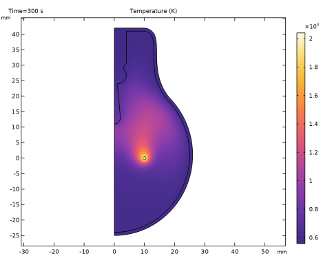
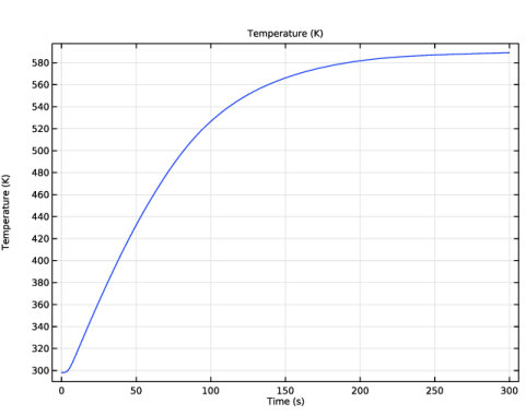
In the tree, select Study 1/Solution 1 (sol1) > Heat Transfer in Solids and Fluids > Temperature (ht).
|
|
4
|
Click the Add Result Template button in the window toolbar.
|
|
5
|
|
1
|
|
2
|
|
3
|
|
4
|
|
5
|
|
6
|
|
7
|
|
1
|
|
2
|
|
3
|
|
4
|
|
5
|
|
1
|
|
2
|
|
3
|
|
4
|
|
1
|
|
2
|
|
3
|
|
4
|
|
5
|
|
6
|
|
7
|
|
8
|
|
1
|
|
2
|
|
3
|
|
4
|
|
1
|
|
2
|
|
1
|
|
2
|
|
3
|
|
4
|
Click Replace Expression in the upper-right corner of the y-Axis Data section. From the menu, choose Component 1 (comp1) > Heat Transfer in Solids and Fluids > Temperature > T - Temperature - K.
|
|
5
|
|
1
|
|
2
|
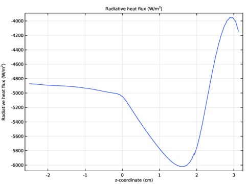
In the Settings window for 1D Plot Group, type Radiative Heat Flux Along z-Coordinate in the Label text field.
|
|
3
|
|
1
|
|
2
|
|
3
|
|
4
|
Click Replace Expression in the upper-right corner of the y-Axis Data section. From the menu, choose Component 1 (comp1) > Surface-to-Surface Radiation > Radiative heat flux > rad.rflux - Radiative heat flux - W/m².
|
|
5
|
Click Replace Expression in the upper-right corner of the x-Axis Data section. From the menu, choose Component 1 (comp1) > Geometry > Coordinate > z - z-coordinate.
|
|
6
|
|
7
|
|
1
|
|
2
|
|
3
|
|
4
|
|
5
|
Click Replace Expression in the upper-right corner of the Expressions section. From the menu, choose Component 1 (comp1) > Surface-to-Surface Radiation > Radiative heat flux > rad.rflux - Radiative heat flux - W/m².
|
|
6
|
Click
|
|
1
|
Go to the Table 1 window.
|
|
1
|
|
2
|
|
1
|
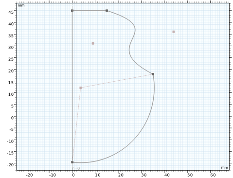
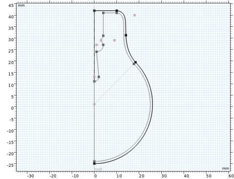
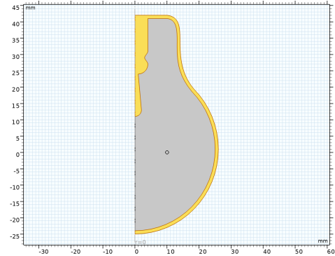
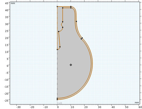
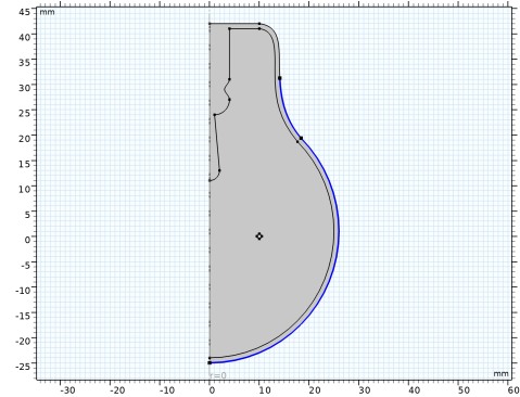
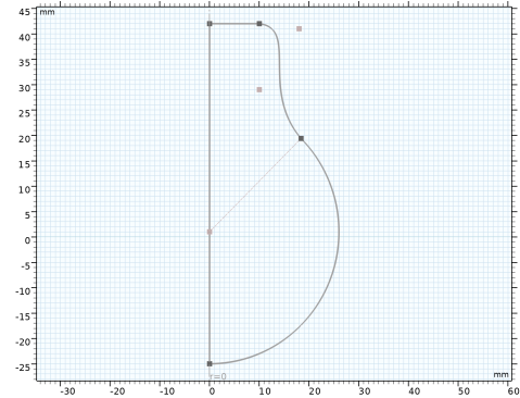
In the Sketch toolbar, click Polygon, then in the Graphics window place the first vertex by clicking on the centerline close to the top of the canvas.
|
|
5
|
To switch drawing a circular arc, right-click in the Graphics window, and from the context menu choose Circular Arc, then choose Start, Center, Angle.
|
|
1
|
In the Model Builder window, expand the Component 1 (comp1) > Geometry 1 > Composite Curve 1 (cc1) node, then click Polygon 1 (pol1).
|
|
2
|
|
1
|
|
2
|
Since the coordinates of the first control point have already been adjusted by editing pol1 change the remaining entries, only.
|
|
1
|
|
2
|
|
3
|
|
4
|
|
5
|
|
6
|
|
7
|
|
8
|
Click
|
|
1
|
|
2
|
|
3
|
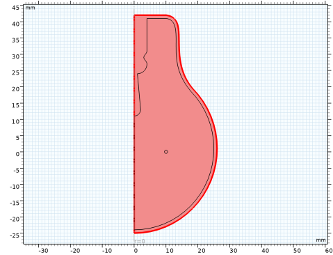
Select the Resulting objects selection checkbox.
|
|
4
|
From the Show in physics list, choose Off. With this setting the selection is available only as input for features in the geometry sequence. This way you can keep only the relevant selections in the list of selections when you are defining, for example, physics and mesh features.
|
|
1
|
|
2
|
|
3
|
|
1
|
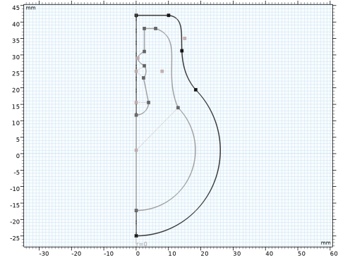
In the Model Builder window, expand the Component 1 (comp1) > Geometry 1 > Composite Curve 2 (cc2) node, then click Polygon 1 (pol1).
 |
|
2
|
|
3
|
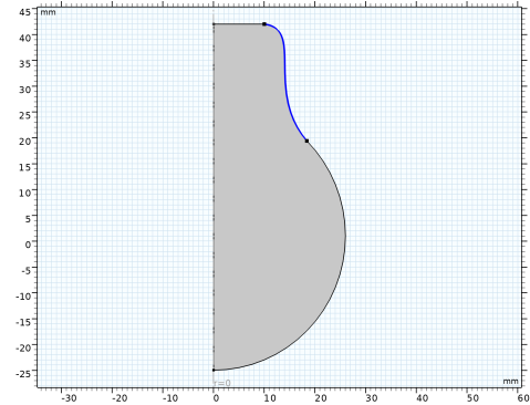
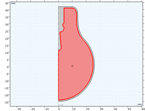
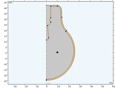
Right-click in the Graphics window and select Polygon. Start to draw an edge perpendicular to the rotation axis. Its first vertex is located inward from the start vertex of the outer shape.
|
|
4
|
Continue with a Cubic Bézier polygon. Try to follow the outer shape.
|
|
5
|
|
6
|
Draw a Polygon up along the centerline to about halfway up the geometry.
|
|
7
|
|
8
|
Use the Polygon tool to draw an edge that tilts toward the centerline.
|
|
9
|
Draw another Circular Arc that curves away from then back toward the centerline. The start and end vertices can be aligned vertically.
|
|
10
|
Switch to an Interpolation Curve to create a curved segment that first curves toward the centerline then away. Use the Interpolation Points option to define the curve, and add one interpolation point. Try to align the start and end vertices vertically.
|
|
11
|
Close the shape with a vertical edge, using the Polygon tool.
|
|
12
|
|
1
|
|
2
|
Since the coordinates of the first control point have already been adjusted by editing pol1 change the remaining entries, only.
|
|
4
|
|
5
|
|
1
|
|
2
|
|
3
|
|
4
|
|
5
|
|
1
|
|
2
|
|
1
|
|
2
|
|
3
|
|
4
|
|
5
|
|
6
|
|
1
|
|
2
|
|
1
|
|
2
|
|
3
|
|
4
|
|
5
|
|
6
|
|
7
|
|
1
|
|
2
|
|
4
|
Locate the End Conditions section. From the Condition at starting point list, choose Tangent direction.
|
|
5
|
|
6
|
|
7
|
|
8
|
|
9
|
|
1
|
|
2
|
|
3
|
|
4
|
Locate the Selections of Resulting Entities section. Select the Resulting objects selection checkbox.
|
|
5
|
|
1
|
|
2
|
|
3
|
|
4
|
|
5
|
Locate the Selections of Resulting Entities section. Select the Resulting objects selection checkbox.
|
|
6
|
|
7
|
|
8
|
|
1
|
|
2
|
Go to the Selection List window.
|
|
3
|
|
4
|
|
5
|
|
1
|
|
2
|
|
3
|
|
1
|
|
2
|
|
3
|
|
4
|
|
5
|
Click OK.
|
|
6
|
|
7
|
|
8
|
|
9
|
|
1
|
|
2
|
|
3
|
|
4
|
|
5
|
|
1
|
|
2
|
|
3
|
|
4
|
|
5
|
Click OK.
|
|
6
|
|
7
|
|
8
|
|
9
|
|
1
|
|
2
|
|
3
|
|
4
|
|
5
|
|
6
|
Click OK.
|
|
7
|
|
8
|
|
9
|
|
10
|
|
1
|
|
2
|
|
3
|
|
4
|
|
1
|
|
2
|
Click in the Graphics window and then press Ctrl+D to clear all objects.
|
|
3
|
|
4
|
|
5
|
|
6
|
|
7
|
Click OK.
|
|
8
|