|
|
|
|
1
|
|
2
|
In the Select Physics tree, select Fluid Flow > Single-Phase Flow > Turbulent Flow > Turbulent Flow, Low Re k-ε (spf).
|
|
3
|
Click Add.
|
|
4
|
Click
|
|
5
|
In the Select Study tree, select Preset Studies for Selected Physics Interfaces > Stationary with Initialization.
|
|
6
|
Click
|
|
1
|
|
2
|
Browse to the model’s Application Libraries folder and double-click the file evaporative_cooling_geom_sequence.mph.
|
|
3
|
|
4
|
|
5
|
|
1
|
|
2
|
Go to the Add Material window.
|
|
3
|
|
4
|
Click the Add to Component button in the window toolbar.
|
|
5
|
|
1
|
|
2
|
|
3
|
|
5
|
Click
|
|
6
|
|
7
|
Click OK.
|
|
1
|
|
3
|
|
4
|
|
1
|
|
1
|
|
1
|
|
2
|
|
3
|
|
4
|
|
1
|
|
3
|
|
4
|
Click the Predefined button.
|
|
5
|
|
6
|
Click
|
|
1
|
|
2
|
|
3
|
|
4
|
|
6
|
|
7
|
Locate the Element Size Parameters section.
|
|
8
|
|
1
|
|
2
|
|
3
|
|
1
|
|
2
|
|
3
|
|
1
|
In the Model Builder window, expand the Boundary Layers 1 node, then click Boundary Layer Properties 1.
|
|
2
|
|
3
|
|
4
|
|
1
|
|
2
|
|
3
|
Click
|
|
4
|
|
5
|
Click OK.
|
|
6
|
|
8
|
Click
|
|
1
|
|
2
|
|
3
|
|
1
|
|
2
|
Go to the Add Physics window.
|
|
3
|
|
4
|
Find the Physics interfaces in study subsection. In the table, clear the Solve checkbox for Study 1.
|
|
5
|
Click the Add to Component 1 button in the window toolbar.
|
|
6
|
|
1
|
|
1
|
|
2
|
Go to the Add Material window.
|
|
3
|
|
4
|
Click the Add to Component button in the window toolbar.
|
|
2
|
|
3
|
Click
|
|
4
|
|
5
|
Click OK.
|
|
1
|
|
2
|
|
3
|
|
4
|
|
5
|
|
6
|
Click OK.
|
|
1
|
Go to the Add Material window.
|
|
2
|
|
3
|
Click the Add to Component button in the window toolbar.
|
|
4
|
|
1
|
|
2
|
|
1
|
|
1
|
|
2
|
In the Settings window for Convectively Enhanced Conductivity, locate the Convectively Enhanced Conductivity section.
|
|
3
|
|
4
|
|
5
|
|
1
|
|
2
|
|
3
|
|
1
|
|
1
|
|
1
|
|
2
|
|
1
|
|
3
|
|
4
|
|
5
|
|
1
|
|
2
|
|
3
|
|
1
|
In the Model Builder window, under Component 1 (comp1) > Moisture Transport in Air (mt) click Initial Values 1.
|
|
2
|
|
3
|
|
1
|
|
3
|
|
4
|
|
1
|
|
3
|
|
4
|
|
1
|
|
1
|
|
3
|
|
4
|
|
1
|
In the Model Builder window, under Component 1 (comp1) > Multiphysics click Heat and Moisture 1 (ham1).
|
|
2
|
|
3
|
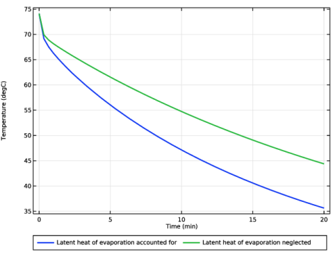
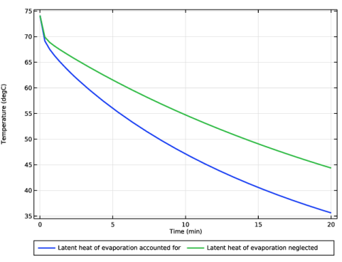
Clear the Include latent heat source on surfaces checkbox.
|
|
1
|
|
2
|
|
3
|
Select the Boussinesq approximation checkbox.
|
|
1
|
|
1
|
|
2
|
In the Settings window for Wall Distance Initialization, locate the Physics and Variables Selection section.
|
|
3
|
In the Solve for column of the table, under Component 1 (comp1) > Multiphysics, clear the checkboxes for Nonisothermal Flow 1 (nitf1) and Moisture Flow 1 (mf1).
|
|
1
|
|
2
|
|
3
|
In the Solve for column of the table, under Component 1 (comp1) > Multiphysics, clear the checkboxes for Nonisothermal Flow 1 (nitf1) and Moisture Flow 1 (mf1).
|
|
1
|
|
2
|
Go to the Add Study window.
|
|
3
|
Find the Physics interfaces in study subsection. In the table, clear the Solve checkbox for Turbulent Flow, Low Re k-ε (spf).
|
|
4
|
|
5
|
Click the Add Study button in the window toolbar.
|
|
6
|
|
1
|
|
2
|
|
3
|
|
4
|
|
5
|
Click to expand the Values of Dependent Variables section. Find the Values of variables not solved for subsection. From the Settings list, choose User controlled.
|
|
6
|
|
7
|
|
1
|
|
2
|
|
3
|
|
4
|
|
5
|
|
6
|
|
7
|
Right-click Study 2 : No Latent Heat Source > Solver Configurations > Solution 3 (sol3) > Time-Dependent Solver 1 and choose Fully Coupled.
|
|
8
|
|
9
|
|
1
|
|
2
|
|
1
|
|
2
|
|
1
|
|
2
|
|
1
|
|
2
|
|
3
|
|
4
|
Locate the Coloring and Style section. Find the Point style subsection. From the Color list, choose White.
|
|
6
|
|
7
|
|
8
|
|
9
|
|
1
|
|
2
|
|
3
|
|
4
|
Locate the Data section. From the Dataset list, choose Study 2 : No Latent Heat Source/Solution 3 (sol3).
|
|
1
|
|
2
|
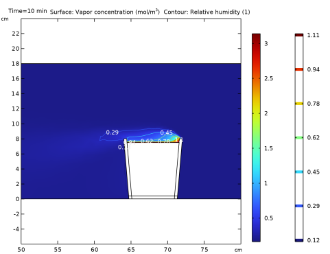
In the Settings window for 2D Plot Group, type Moisture Concentration and Relative Humidity in the Label text field.
|
|
3
|
Locate the Plot Settings section. From the View list, choose New view to generate a dedicated view for this plot.
|
|
4
|
|
5
|
|
1
|
|
2
|
In the Settings window for Surface, click Replace Expression in the upper-right corner of the Expression section. From the menu, choose Component 1 (comp1) > Moisture Transport in Air > Moist air properties > mt.cv - Vapor concentration - mol/m³.
|
|
1
|
|
2
|
|
3
|
|
4
|
|
5
|
|
6
|
|
7
|
Select the Level labels checkbox.
|
|
8
|
|
9
|
|
10
|
|
1
|
|
2
|
|
3
|
Locate the Data section. From the Dataset list, choose Study 2 : No Latent Heat Source/Solution 3 (sol3).
|
|
5
|
Click Replace Expression in the upper-right corner of the Expressions section. From the menu, choose Component 1 (comp1) > Heat Transfer in Moist Air > Temperature > T - Temperature - K.
|
|
6
|
Click
|
|
1
|
Go to the Table 1 window.
|
|
2
|
Click the Table Graph button in the window toolbar.
|
|
1
|
|
2
|
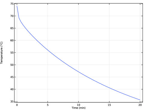
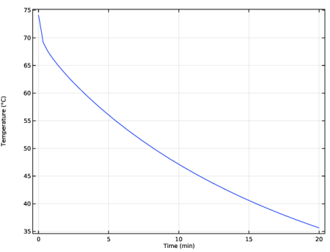
In the Settings window for 1D Plot Group, type Average Water Temperature over Time in the Label text field.
|
|
1
|
|
2
|
In the Settings window for Surface Integration, type Amount of Evaporated Water in the Label text field.
|
|
3
|
Locate the Data section. From the Dataset list, choose Study 2 : No Latent Heat Source/Solution 3 (sol3).
|
|
5
|
Locate the Expressions section. In the table, enter the following settings:
|
|
6
|
|
7
|
|
1
|
Go to the Table 2 window.
|
|
1
|
|
1
|
|
2
|
|
3
|
In the Solve for column of the table, under Component 1 (comp1) > Multiphysics, clear the checkbox for Heat and Moisture 2 (ham2).
|
|
1
|
|
2
|
|
3
|
In the Solve for column of the table, under Component 1 (comp1) > Multiphysics, clear the checkbox for Heat and Moisture 2 (ham2).
|
|
1
|
|
2
|
Go to the Add Study window.
|
|
3
|
Find the Physics interfaces in study subsection. In the table, clear the Solve checkbox for Turbulent Flow, Low Re k-ε (spf).
|
|
4
|
|
5
|
Click the Add Study button in the window toolbar.
|
|
6
|
|
1
|
|
2
|
|
3
|
|
4
|
|
5
|
Locate the Physics and Variables Selection section. In the Solve for column of the table, under Component 1 (comp1) > Multiphysics, clear the checkbox for Heat and Moisture 1 (ham1).
|
|
6
|
Locate the Values of Dependent Variables section. Find the Values of variables not solved for subsection. From the Settings list, choose User controlled.
|
|
7
|
|
8
|
|
1
|
|
2
|
|
3
|
|
4
|
|
5
|
|
6
|
|
7
|
Right-click Study 3 : Latent Heat Source > Solver Configurations > Solution 4 (sol4) > Time-Dependent Solver 1 and choose Fully Coupled.
|
|
8
|
|
9
|
|
1
|
|
2
|
|
1
|
|
2
|
|
3
|
|
4
|
|
5
|
|
1
|
|
2
|
|
3
|
|
1
|
|
2
|
|
1
|
Go to the Table 1 window.
|
|
2
|
Click the Clear Table button in the window toolbar.
|
|
1
|
|
2
|
|
3
|
|
4
|
|
5
|
Click
|
|
1
|
Go to the Table 1 window.
|
|
2
|
Click the Table Graph button in the window toolbar.
|
|
1
|
|
2
|
|
1
|
Go to the Table 1 window.
|
|
2
|
Click the Table Graph button in the window toolbar.
|
|
1
|
|
2
|
|
3
|
|
4
|
|
1
|
|
2
|
|
3
|
|
4
|
|
5
|
|
6
|
|
1
|
|
2
|
|
3
|
Locate the Data section. From the Dataset list, choose Study 3 : Latent Heat Source/Solution 4 (sol4).
|
|
4
|
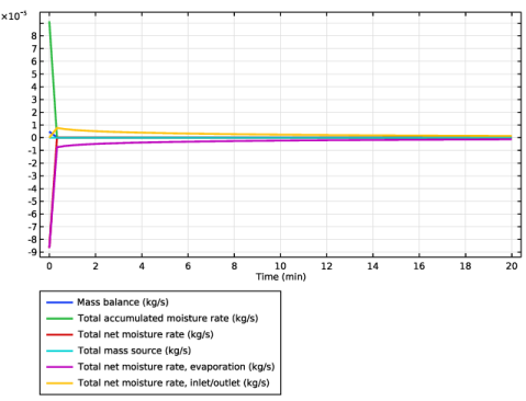
Click Replace Expression in the upper-right corner of the Expressions section. From the menu, choose Component 1 (comp1) > Moisture Transport in Air > Mass balance > mt.massBalance - Mass balance - kg/s.
|
|
5
|
Click Add Expression in the upper-right corner of the Expressions section. From the menu, choose Component 1 (comp1) > Moisture Transport in Air > Mass balance > mt.dwcInt - Total accumulated moisture rate - kg/s.
|
|
6
|
Click Add Expression in the upper-right corner of the Expressions section. From the menu, choose Component 1 (comp1) > Moisture Transport in Air > Mass balance > mt.ntfluxInt - Total net moisture rate - kg/s.
|
|
7
|
Click Add Expression in the upper-right corner of the Expressions section. From the menu, choose Component 1 (comp1) > Moisture Transport in Air > Mass balance > mt.GInt - Total mass source - kg/s.
|
|
8
|
Click Add Expression in the upper-right corner of the Expressions section. From the menu, choose Component 1 (comp1) > Moisture Transport in Air > Mass balance > Net mass flows, boundary features > mt.ws1.ntfluxInt - Total net moisture rate - kg/s.
|
|
9
|
Click Add Expression in the upper-right corner of the Expressions section. From the menu, choose Component 1 (comp1) > Moisture Transport in Air > Mass balance > Net mass flows, boundary features > mt.ifl1.ntfluxInt - Total net moisture rate - kg/s.
|
|
10
|
Locate the Expressions section. In the table, enter the following settings:
|
|
11
|
Click
|
|
1
|
Go to the Table 3 window.
|
|
2
|
Click the Table Graph button in the window toolbar.
|
|
1
|
|
2
|
|
3
|
|
4
|
|
5
|
|
1
|
|
2
|
|
3
|
Select the Show legends checkbox.
|
|
4
|