|
|
|

|
ρ (kg/m3)
|
|||
|
Cp (J/(kg·K))
|
|||
|
k (W/(m·K))
|
|||
|
μ (N·s/m2)
|
|
1
|
|
2
|
|
3
|
Click Add.
|
|
4
|
Click
|
|
5
|
|
6
|
Click
|
|
1
|
|
2
|
|
3
|
Click
|
|
4
|
Browse to the model’s Application Libraries folder and double-click the file continuous_casting_apparent_heat_capacity_parameters.txt.
|
|
1
|
|
2
|
|
3
|
|
4
|
|
5
|
|
6
|
Browse to the model’s Application Libraries folder and double-click the file continuous_casting_apparent_heat_capacity_variables.txt.
|
|
1
|
|
2
|
|
3
|
|
4
|
|
5
|
|
6
|
|
1
|
|
2
|
|
3
|
|
4
|
|
5
|
|
6
|
|
1
|
|
2
|
|
3
|
|
4
|
|
5
|
|
6
|
Click to expand the Layers section. In the table, enter the following settings:
|
|
7
|
|
8
|
|
1
|
|
2
|
|
4
|
|
5
|
|
1
|
|
2
|
|
3
|
Locate the Material Contents section. In the table, enter the following settings:
|
|
1
|
|
2
|
|
3
|
|
4
|
Locate the Material Contents section. In the table, enter the following settings:
|
|
1
|
|
2
|
|
3
|
Specify the u vector as
|
|
1
|
|
3
|
|
4
|
From the list, choose Pressure.
|
|
1
|
|
3
|
|
4
|
From the list, choose Velocity.
|
|
5
|
|
6
|
|
1
|
|
3
|
|
4
|
|
1
|
|
2
|
|
3
|
|
4
|
|
1
|
|
2
|
|
3
|
|
1
|
|
2
|
|
3
|
|
4
|
|
5
|
|
6
|
|
7
|
|
1
|
In the Model Builder window, under Component 1 (comp1) > Heat Transfer in Fluids (ht) click Initial Values 1.
|
|
2
|
|
3
|
|
1
|
|
3
|
|
4
|
|
1
|
|
3
|
|
4
|
|
5
|
|
6
|
|
1
|
|
3
|
|
4
|
|
5
|
|
6
|
|
1
|
|
3
|
|
4
|
|
5
|
|
6
|
|
1
|
|
1
|
|
3
|
In the Settings window for Surface-to-Ambient Radiation, locate the Surface-to-Ambient Radiation section.
|
|
4
|
|
5
|
|
1
|
|
2
|
|
3
|
|
1
|
|
2
|
Click Yes to confirm.
|
|
1
|
|
3
|
|
4
|
|
5
|
|
1
|
|
2
|
|
3
|
Clear the Generate default plots checkbox.
|
|
1
|
|
2
|
|
3
|
Select the Auxiliary sweep checkbox.
|
|
4
|
Click
|
|
1
|
|
2
|
|
3
|
|
1
|
|
2
|
|
3
|
In the Model Builder window, expand the Study 1 > Solver Configurations > Solution 1 (sol1) > Stationary Solver 2 node, then click Adaptive Mesh Refinement.
|
|
4
|
|
5
|
Clear the Allow coarsening checkbox.
|
|
6
|
|
1
|
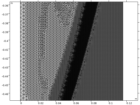
In the Model Builder window, expand the Component 1 (comp1) > Meshes node, then click Level 2 Adapted Mesh 2.
|
|
2
|
|
3
|
Click the Zoom Box button in the Graphics toolbar and then use the mouse to zoom in on the transition zone where the mesh is the densest.
|
|
1
|
|
2
|
Go to the Add Study window.
|
|
3
|
|
4
|
Click the Add Study button in the window toolbar.
|
|
5
|
|
1
|
|
2
|
|
3
|
Find the Initial values of variables solved for subsection. From the Settings list, choose User controlled.
|
|
4
|
|
5
|
|
6
|
|
7
|
Click
|
|
1
|
|
2
|
|
3
|
Right-click Study 2 > Solver Configurations > Solution 7 (sol7) > Stationary Solver 1 and choose Fully Coupled.
|
|
4
|
|
1
|
|
2
|
|
3
|
|
1
|
|
2
|
|
3
|
|
4
|
|
5
|
Locate the Coloring and Style section. Find the Point style subsection. From the Type list, choose Arrow.
|
|
6
|
|
1
|
|
2
|
|
3
|
|
1
|
|
2
|
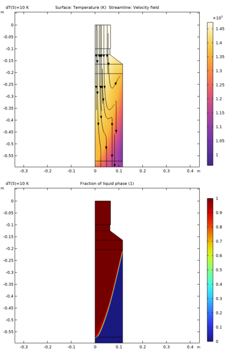
In the Settings window for Surface, click Replace Expression in the upper-right corner of the Expression section. From the menu, choose Component 1 (comp1) > Definitions > Variables > alpha - Fraction of liquid phase - 1.
|
|
3
|
|
1
|
|
2
|
|
1
|
|
2
|
|
3
|
|
4
|
|
5
|
|
6
|
Locate the Coloring and Style section. Find the Point style subsection. From the Type list, choose Arrow.
|
|
7
|
|
1
|
|
2
|
|
3
|
|
1
|
|
2
|
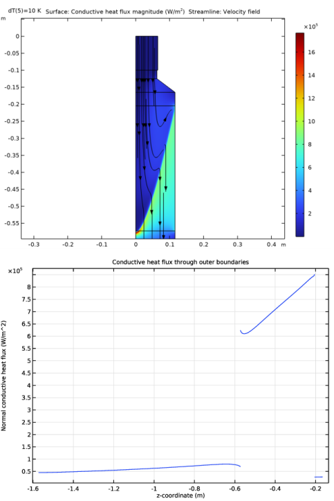
In the Settings window for Surface, click Replace Expression in the upper-right corner of the Expression section. From the menu, choose Component 1 (comp1) > Heat Transfer in Fluids > Domain fluxes > ht.dfluxMag - Conductive heat flux magnitude - W/m².
|
|
3
|
|
1
|
|
2
|
|
3
|
|
4
|
|
5
|
|
6
|
Locate the Coloring and Style section. Find the Point style subsection. From the Type list, choose Arrow.
|
|
7
|
|
1
|
|
2
|
In the Settings window for 1D Plot Group, type Conductive Heat Flux through Outer Boundaries in the Label text field.
|
|
3
|
|
4
|
|
5
|
|
6
|
|
7
|
Locate the Plot Settings section.
|
|
8
|
|
9
|
Select the y-axis label checkbox. In the associated text field, type Normal conductive heat flux (W/m^2).
|
|
1
|
|
3
|
In the Settings window for Line Graph, click Replace Expression in the upper-right corner of the y-Axis Data section. From the menu, choose Component 1 (comp1) > Heat Transfer in Fluids > Boundary fluxes > ht.ndflux - Normal conductive heat flux - W/m².
|
|
4
|
Click Replace Expression in the upper-right corner of the x-Axis Data section. From the menu, choose Component 1 (comp1) > Geometry > Coordinate > z - z-coordinate.
|
|
5
|
|
6
|
|
7
|
Click to collapse the Quality section. In the Conductive Heat Flux through Outer Boundaries toolbar, click
|
|
1
|
|
2
|
|
3
|
|
4
|
|
5
|
|
1
|
|
2
|
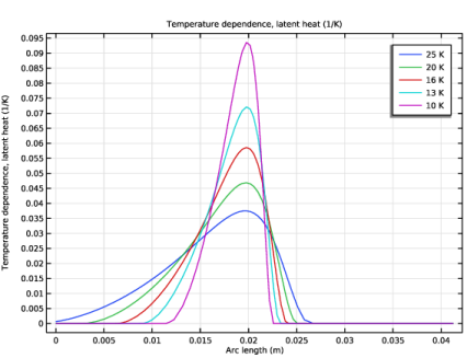
In the Settings window for 1D Plot Group, type Temperature Dependence, Latent Heat in the Label text field.
|
|
3
|
|
1
|
|
2
|
In the Settings window for Line Graph, click Replace Expression in the upper-right corner of the y-Axis Data section. From the menu, choose Component 1 (comp1) > Definitions > Variables > D - Temperature dependence, latent heat - 1/K.
|
|
3
|
|
4
|