PDF

Contact Switch
Introduction
A contact switch is used to regulate whether or not an electric current is passing from a power source into an electrical device. These switches are found in many types of equipment and they are used to control, for example, the power output from a wall socket into a device when it is plugged in; the currents passing across the circuit board of a computer; or the electricity powering a light bulb when the switch is flipped on. Because of their prevalence, simulating contact switches is a fundamental step in designing electronic applications.
The working principle behind a contact switch is simple: two conductive pieces of metal with an electric-voltage difference across them are brought into contact, allowing a current to flow between them. The metallic surfaces of the two components that touch one another are called contacts, and when the connection between the two contacts is broken, the current stops flowing.
The current flow between the two contacts contributes to an increase in temperature in the switch due to the Joule heating effect.
Figure 1: A contact switch.
The heating of the contact switch can change the material properties of the metal as well as the surface area of contact, and therefore is an important effect to consider when modeling the switch. Letting the temperature become too high can even cause the switch to burn out, meaning the switch is no longer functional. Therefore, it is important to analyze its current-carrying capability in order to prevent overheating. It is also important to consider that when the two metallic pieces come into contact, the surfaces touching each other experience a mechanical pressure or contact pressure. This mechanical pressure on the contacts can alter the electrical and thermal properties of the material locally around the region surrounding the contacts. Therefore, in order to accurately simulate the current-carrying capability and temperature rise in the switch, it is important to take a more comprehensive approach in the simulation and incorporate the effect of contact pressure to compute the electrical and thermal conductance of the contact surfaces.This tutorial illustrates how to implement a multiphysics contact. It models the thermal and electrical behavior of two contacting parts of a switch. The electric current and the heat cross from one part to the other only through the contact area.
The contact switch device has a cylindrical body and plate hook shapes at the contact area (see Figure 1). There, the thermal and electrical apparent resistances are coupled to the mechanical contact pressure at the interface, which the application solves.
The initial temperature is equal to the external room temperature. A potential difference between the left and right parts leads to heating through the Joule effect.
Model Definition
The geometry of the switch is shown in Figure 2. Only half of the device is represented due to symmetry considerations.
Figure 2: Switch geometry.
The switch is made of copper, with two fixed cylindrical elements and a central region where the contacts are located. On the end of each contact are plate hooks that enable contact between the two pieces. In the simulation, an electric potential of 1 mV is applied to the left side of the switch, while the right side is grounded.
The thermal and electrical contact conductances are assumed to be related only to the contact pressure.
The exposed surfaces of the switch lose heat due to their interaction with air via natural convection. In the simulation, this is modeled by specifying a heat transfer coefficient and the ambient temperature of the surrounding air (a more ambitious simulation might also include the fluid flow of the air). The application first solves for structural contact to obtain the contact pressure on the contact surfaces. These results are then used to compute the electrical and thermal conductance of the contact’s surfaces in a Joule heating simulation.
Results and Discussion
Figure 3 shows the electric potential distribution, ranging from the grounded right side to the applied 1 mV on the left.
Figure 3: Electric potential profile.
A potential difference across the two components in the switch creates a current flow, which in turn leads to Joule heating. This causes a rise in temperature in the switch. If you leave the switch on for a while, temperature distribution in the switch reaches an equilibrium. Figure 4 shows the temperature distribution in the contact switch. In this example, Joule heating causes the temperature in the switch to rise about 5 K above room temperature, although only a small temperature variation is seen within the switch itself.
Figure 4: Temperature distribution.
The internal temperature distribution is almost constant. Introducing the effect of electrical and thermal conductance allows us to predict the temperature rise more accurately. The simulation also shows that the switch gets slightly hotter at the contact region.
Finally, Figure 5 plots the temperature distribution at the contact region. Streamlines show the current density.
Figure 5: Temperature distribution (surface plot) and current density (streamlines) at the contact region.
Application Library path: Heat_Transfer_Module/Thermal_Contact_and_Friction/contact_switch
Modeling Instructions
From the File menu, choose New.
New
In the New window, click  Model Wizard.
Model Wizard
1
In the Model Wizard window, click  3D.
2
In the Select Physics tree, select Structural Mechanics > Solid Mechanics (solid).
3
Click Add.
4
In the Select Physics tree, select Heat Transfer > Electromagnetic Heating > Joule Heating.
5
Click Add.
6
Click  Study.
7
In the Select Study tree, select General Studies > Stationary.
8
Geometry 1
The model geometry is provided in a separate MPHBIN file. If you prefer to create it from scratch, follow the steps outlined in the Geometry Modeling Instructions. Note that a license for the Design Module is required to create the geometry. Otherwise, you can import the geometry as follows:
Import 1 (imp1)
1
In the Geometry toolbar, click  Import.
2
In the Settings window for Import, locate the Source section.
3
Click  Browse.
4
5
Click  Import.
Form Union (fin)
1
In the Model Builder window, under Component 1 (comp1) > Geometry 1 click Form Union (fin).
2
In the Settings window for Form Union/Assembly, locate the Form Union/Assembly section.
3
From the Action list, choose Form an assembly.
4
From the Pair type list, choose Contact pair.
5
Clear the Create pairs checkbox.
6
In the Geometry toolbar, click  Build All.
Definitions
Contact Pair 1 (p1)
1
In the Definitions toolbar, click  Pairs and choose Contact Pair.
2
3
In the Settings window for Pair, locate the Destination Boundaries section.
4
Click to select the  Activate Selection toggle button.
5
Add Material
1
In the Materials toolbar, click  Add Material to open the Add Material window.
2
Go to the Add Material window.
3
In the tree, select Built-in > Copper.
4
Click the Add to Component button in the window toolbar.
5
In the Materials toolbar, click  Add Material to close the Add Material window.
Solid Mechanics (solid)
Fixed Constraint 1
1
In the Physics toolbar, click  Boundaries and choose Fixed Constraint.
2
Symmetry 1
1
In the Physics toolbar, click  Boundaries and choose Symmetry.
2
Contact 1
1
In the Model Builder window, click Contact 1.
2
In the Settings window for Contact, locate the Contact Method section.
3
From the list, choose Augmented Lagrangian.
Heat Transfer in Solids (ht)
In the Model Builder window, under Component 1 (comp1) click Heat Transfer in Solids (ht).
Heat Flux 1
1
In the Physics toolbar, click  Boundaries and choose Heat Flux.
2
3
In the Settings window for Heat Flux, locate the Heat Flux section.
4
From the Flux type list, choose Convective heat flux.
5
In the h text field, type 2[W/(m^2*K)].
Symmetry 1
1
In the Physics toolbar, click  Boundaries and choose Symmetry.
2
Thermal Contact 1
1
In the Physics toolbar, click  Pairs and choose Thermal Contact.
2
In the Settings window for Thermal Contact, locate the Pair Selection section.
3
4
In the Add dialog, select Contact Pair 1 (p1) in the Pairs list.
5
6
In the Settings window for Thermal Contact, locate the Contact Surface Properties section.
7
From the p list, choose Contact pressure (solid/dcnt1).
Electric Currents (ec)
In the Model Builder window, under Component 1 (comp1) click Electric Currents (ec).
Ground 1
1
In the Physics toolbar, click  Boundaries and choose Ground.
2
Electric Potential 1
1
In the Physics toolbar, click  Boundaries and choose Electric Potential.
2
3
In the Settings window for Electric Potential, locate the Electric Potential section.
4
In the V0 text field, type 1[mV].
Electrical Contact 1
1
In the Physics toolbar, click  Pairs and choose Electrical Contact.
2
In the Settings window for Electrical Contact, locate the Pair Selection section.
3
4
In the Add dialog, select Contact Pair 1 (p1) in the Pairs list.
5
6
In the Settings window for Electrical Contact, locate the Contact Surface Properties section.
7
From the p list, choose Contact pressure (solid/dcnt1).
Mesh 1
Free Tetrahedral 1
In the Mesh toolbar, click  Free Tetrahedral.
Size 1
1
Right-click Free Tetrahedral 1 and choose Size.
2
In the Settings window for Size, locate the Geometric Entity Selection section.
3
From the Geometric entity level list, choose Boundary.
4
5
Locate the Element Size section. Click the Custom button.
6
Locate the Element Size Parameters section.
7
Select the Maximum element size checkbox. In the associated text field, type 5e-4.
Size
1
In the Model Builder window, under Component 1 (comp1) > Mesh 1 click Size.
2
In the Settings window for Size, locate the Element Size section.
3
From the Predefined list, choose Fine.
4
Click  Build All.
Study 1
Solve the model in two steps. The first step only computes for Solid Mechanics while the second solves for Joule Heating (Electric Currents and Heat Transfer in Solids).
Step 1: Stationary
1
In the Model Builder window, under Study 1 click Step 1: Stationary.
2
In the Settings window for Stationary, locate the Physics and Variables Selection section.
3
In the Solve for column of the table, under Component 1 (comp1), clear the checkboxes for Electric Currents (ec) and Heat Transfer in Solids (ht).
4
In the Solve for column of the table, under Component 1 (comp1) > Multiphysics, clear the checkbox for Electromagnetic Heating 1 (emh1).
Step 2: Stationary 2
1
In the Study toolbar, click  Stationary.
2
In the Settings window for Stationary, locate the Physics and Variables Selection section.
3
In the Solve for column of the table, under Component 1 (comp1), clear the checkbox for Solid Mechanics (solid).
4
In the Study toolbar, click  Compute.
Results
Stress (solid)
In this first default plot, the switch is slightly deformed due to the contact pressure. The von Mises stress is located at the switch base and at the contact area.
Follow the next steps to visualize the third and fifth default plots as in Figure 3 and Figure 4.
Mirror 3D 1
1
In the Model Builder window, expand the Results > Datasets node.
2
Right-click Results > Datasets and choose More 3D Datasets > Mirror 3D.
3
In the Settings window for Mirror 3D, locate the Plane Data section.
4
From the Plane list, choose xy-planes.
Electric Potential (ec)
1
In the Model Builder window, under Results click Electric Potential (ec).
2
In the Settings window for 3D Plot Group, locate the Data section.
3
From the Dataset list, choose Mirror 3D 1.
4
In the Electric Potential (ec) toolbar, click  Plot.
Temperature (ht)
1
In the Model Builder window, click Temperature (ht).
2
In the Settings window for 3D Plot Group, locate the Data section.
3
From the Dataset list, choose Mirror 3D 1.
4
Locate the Plot Settings section. From the Frame list, choose Spatial  (x, y, z).
5
In the Temperature (ht) toolbar, click  Plot.
To observe the temperature and current density only at the contact region (Figure 5), proceed as follows.
Surface 1
1
In the Results toolbar, click  More Datasets and choose Surface.
2
In the Settings window for Surface, locate the Parameterization section.
3
From the x- and y-axes list, choose xy-plane.
4
Temperature (Contact Region)
1
In the Results toolbar, click  2D Plot Group.
2
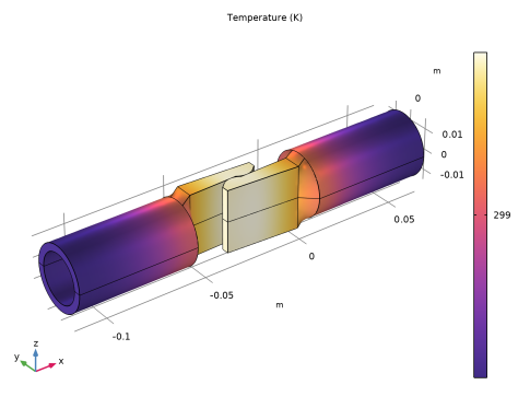
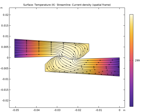
In the Settings window for 2D Plot Group, type Temperature (Contact Region) in the Label text field.
3
Locate the Plot Settings section. From the Frame list, choose Spatial  (x, y, z).
Surface 1
1
In the Temperature (Contact Region) toolbar, click  Surface.
2
In the Settings window for Surface, click Replace Expression in the upper-right corner of the Expression section. From the menu, choose Component 1 (comp1) > Heat Transfer in Solids > Temperature > T - Temperature - K.
3
Locate the Coloring and Style section. From the Color table list, choose HeatCameraLight.
Temperature (Contact Region)
In the Model Builder window, click Temperature (Contact Region).
Streamline 1
1
In the Temperature (Contact Region) toolbar, click  Streamline.
2
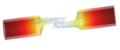
In the Settings window for Streamline, click Replace Expression in the upper-right corner of the Expression section. From the menu, choose Component 1 (comp1) > Electric Currents > Currents and charge > ec.Jx,ec.Jy - Current density (spatial frame).
3
Locate the Streamline Positioning section. From the Positioning list, choose Uniform density.
4
In the Density level text field, type 8.
5
Locate the Coloring and Style section. Find the Point style subsection. From the Type list, choose Arrow.
6
In the Temperature (Contact Region) toolbar, click  Plot.
Geometry Modeling Instructions
Follow these steps to create the geometry for the contact switch model. Note that a license for the Design Module is required for some geometric operations.
From the File menu, choose New.
New
In the New window, click  Model Wizard.
Model Wizard
1
In the Model Wizard window, click  3D.
2
Geometry 1
1
In the Model Builder window, under Component 1 (comp1) click Geometry 1.
2
In the Settings window for Geometry, locate the Advanced section.
3
From the Geometry representation list, choose CAD kernel.
4
Select the Design Module Boolean operations checkbox.
Work Plane 1 (wp1)
In the Geometry toolbar, click  Work Plane.
Work Plane 1 (wp1) > Plane Geometry
In the Model Builder window, click Plane Geometry.
Work Plane 1 (wp1) > Polygon 1 (pol1)
1
In the Work Plane toolbar, click  Polygon.
2
In the Settings window for Polygon, locate the Coordinates section.
3
4
Locate the Object Type section. From the Type list, choose Open curve.
5
Click  Build Selected.
6
Click the  Zoom Extents button in the Graphics toolbar.
Work Plane 1 (wp1) > Circular Arc 1 (ca1)
1
In the Work Plane toolbar, click  More Primitives and choose Circular Arc.
2
In the Settings window for Circular Arc, locate the Properties section.
3
From the Specify list, choose Endpoints and radius.
4
Locate the Starting Point section. In the xw text field, type -33.6[mm].
5
In the yw text field, type -0.94[mm].
6
Locate the Endpoint section. In the xw text field, type -24.4[mm].
7
In the yw text field, type -0.68[mm].
8
Locate the Radius section. In the Radius text field, type 7.2[mm].
9
Locate the Angles section. Select the Clockwise checkbox.
10
Click  Build Selected.
Work Plane 1 (wp1) > Convert to Solid 1 (csol1)
1
In the Work Plane toolbar, click  Conversions and choose Convert to Solid.
2
Click in the Graphics window and then press Ctrl+A to select both objects.
3
Click the  Zoom Extents button in the Graphics toolbar.
4
In the Settings window for Convert to Solid, click  Build Selected.
Work Plane 1 (wp1)
In the Model Builder window, collapse the Component 1 (comp1) > Geometry 1 > Work Plane 1 (wp1) node.
Extrude 1 (ext1)
1
In the Model Builder window, right-click Geometry 1 and choose Extrude.
2
In the Settings window for Extrude, locate the Distances section.
3
4
Select the Reverse direction checkbox.
5
Click  Build Selected.
6
Click the  Zoom Extents button in the Graphics toolbar.
Work Plane 2 (wp2)
1
In the Geometry toolbar, click  Work Plane.
2
In the Settings window for Work Plane, locate the Plane Definition section.
3
From the Plane list, choose yz-plane.
4
In the x-coordinate text field, type 6.8[mm].
Work Plane 2 (wp2) > Plane Geometry
In the Model Builder window, click Plane Geometry.
Work Plane 2 (wp2) > Circular Arc 1 (ca1)
1
In the Work Plane toolbar, click  More Primitives and choose Circular Arc.
2
In the Settings window for Circular Arc, locate the Radius section.
3
In the Radius text field, type 15[mm].
4
Locate the Angles section. In the Start angle text field, type -180[deg].
5
In the End angle text field, type 0[deg].
6
Click  Build Selected.
Work Plane 2 (wp2) > Line Segment 1 (ls1)
1
In the Work Plane toolbar, click  More Primitives and choose Line Segment.
2
On the object ca1, select Point 1 only.
3
In the Settings window for Line Segment, locate the Endpoint section.
4
Click to select the  Activate Selection toggle button for End vertex.
5
On the object ca1, select Point 2 only.
6
Click  Build Selected.
Work Plane 2 (wp2) > Convert to Solid 1 (csol1)
1
In the Work Plane toolbar, click  Conversions and choose Convert to Solid.
2
Click in the Graphics window and then press Ctrl+A to select both objects.
3
In the Settings window for Convert to Solid, click  Build Selected.
4
Click the  Zoom Extents button in the Graphics toolbar.
Work Plane 2 (wp2)
In the Model Builder window, collapse the Component 1 (comp1) > Geometry 1 > Work Plane 2 (wp2) node.
Extrude 2 (ext2)
1
In the Model Builder window, right-click Geometry 1 and choose Extrude.
2
In the Settings window for Extrude, locate the Distances section.
3
4
Click  Build Selected.
5
Click the  Zoom Extents button in the Graphics toolbar.
Work Plane 3 (wp3)
1
In the Model Builder window, under Component 1 (comp1) > Geometry 1 right-click Work Plane 2 (wp2) and choose Duplicate.
2
In the Settings window for Work Plane, locate the Plane Definition section.
3
In the x-coordinate text field, type 14.5[mm].
Work Plane 3 (wp3) > Plane Geometry
In the Model Builder window, expand the Work Plane 3 (wp3) node, then click Plane Geometry.
Work Plane 3 (wp3) > Circular Arc 1 (ca1)
1
In the Model Builder window, expand the Work Plane 3 (wp3) > Plane Geometry node, then click Circular Arc 1 (ca1).
2
In the Settings window for Circular Arc, locate the Radius section.
3
In the Radius text field, type 11.45[mm].
Work Plane 3 (wp3)
In the Model Builder window, collapse the Component 1 (comp1) > Geometry 1 > Work Plane 3 (wp3) node.
Extrude 3 (ext3)
1
In the Model Builder window, right-click Geometry 1 and choose Extrude.
2
In the Settings window for Extrude, locate the Distances section.
3
4
Click  Build Selected.
5
Click the  Zoom Extents button in the Graphics toolbar.
Difference 1 (dif1)
1
In the Geometry toolbar, click  Booleans and Partitions and choose Difference.
2
3
In the Settings window for Difference, locate the Difference section.
4
Click to select the  Activate Selection toggle button for Objects to subtract.
5
6
Click  Build Selected.
Line Segment 1 (ls1)
1
In the Geometry toolbar, click  More Primitives and choose Line Segment.
2
On the object ext1, select Point 11 only.
3
In the Settings window for Line Segment, locate the Endpoint section.
4
From the Specify list, choose Coordinates.
5
In the x text field, type 6.8[mm].
6
In the y text field, type 4.2[mm].
7
In the z text field, type -sqrt((15[mm])^2-(4.2[mm])^2).
8
Locate the Assigned Attributes section. Select the Construction geometry checkbox.
Line Segment 2 (ls2)
1
Right-click Line Segment 1 (ls1) and choose Duplicate.
2
In the Settings window for Line Segment, locate the Starting Point section.
3
Click to select the  Activate Selection toggle button for Start vertex.
4
5
On the object ext1, select Point 9 only.
6
Locate the Endpoint section. In the y text field, type -4.2[mm].
7
Click  Build Selected.
Loft 1 (loft1)
1
In the Geometry toolbar, click  Loft.
2
In the Settings window for Loft, click to expand the Start Profile section.
3
Click to select the  Activate Selection toggle button for Start profile.
4
On the object dif1, select Boundary 1 only.
5
Click to expand the End Profile section. Click to select the  Activate Selection toggle button for End profile.
6
On the object ext1, select Boundary 8 only.
7
Click to expand the Guide Curves section. Click to select the  Activate Selection toggle button for Guide objects.
8
Select the objects ls1 and ls2 only.
9
Click  Build Selected.
Rigid Transform 1 (rt1)
1
In the Geometry toolbar, click  Transforms and choose Rigid Transform.
2
3
In the Settings window for Rigid Transform, locate the Displacement section.
4
In the xw text field, type -50.5[mm].
5
Locate the Rotation section. In the Angle text field, type 180[deg].
6
Locate the Input section. Select the Keep input objects checkbox.
7
Click  Build Selected.
8
Click the  Zoom Extents button in the Graphics toolbar.
Intersection 1 (int1)
1
In the Geometry toolbar, click  Booleans and Partitions and choose Intersection.
2
Click in the Graphics window and then press Ctrl+A to select both objects.
3
In the Settings window for Intersection, locate the Intersection section.
4
Select the Keep input objects checkbox.
5
Click  Build Selected.
Extract 1 (extract1)
1
In the Geometry toolbar, click  Extract.
2
In the Settings window for Extract, locate the Entities or Objects to Extract section.
3
From the Geometric entity level list, choose Edge.
4
On the object int1, select Edges 1, 6, 7, and 12 only.
5
From the Input object handling list, choose Remove.
6
Click  Build Selected.
Copy 1 (copy1)
1
In the Geometry toolbar, click  Transforms and choose Copy.
2
Select the object extract1 only.
3
In the Settings window for Copy, click  Build Selected.
Union 1 (uni1)
1
In the Geometry toolbar, click  Booleans and Partitions and choose Union.
2
Select the objects extract1 and loft1 only.
3
In the Settings window for Union, click  Build Selected.
Union 2 (uni2)
1
In the Geometry toolbar, click  Booleans and Partitions and choose Union.
2
Select the objects copy1 and rt1 only.
3
In the Settings window for Union, click  Build Selected.
Form Union (fin)
1
In the Model Builder window, under Component 1 (comp1) > Geometry 1 click Form Union (fin).
2
In the Settings window for Form Union/Assembly, locate the Form Union/Assembly section.
3
From the Action list, choose Form an assembly.
4
Clear the Create pairs checkbox.
Ignore Faces 1 (igf1)
1
In the Geometry toolbar, click  Virtual Operations and choose Ignore Faces.
2
On the object fin, select Boundaries 6, 11, 34, and 39 only.
3
In the Settings window for Ignore Faces, locate the Input section.
4
Clear the Ignore adjacent edges and vertices checkbox.
5
Click  Build Selected.
Ignore Edges 1 (ige1)
1
In the Geometry toolbar, click  Virtual Operations and choose Ignore Edges.
2
On the object igf1, select Edges 12, 23, 79, and 85 only.
3
In the Settings window for Ignore Edges, click  Build Selected.
Ignore Vertices 1 (igv1)
1
In the Geometry toolbar, click  Virtual Operations and choose Ignore Vertices.
2
On the object ige1, select Points 9 and 54 only.
3
In the Geometry toolbar, click  Build All.
4
Click the  Zoom Extents button in the Graphics toolbar.
Convert to COMSOL 1 (ccom1)
1
In the Geometry toolbar, click  Conversions and choose Convert to COMSOL.
2
Click in the Graphics window and then press Ctrl+A to select both objects.
Ignore Vertices 1 (igv1)
1
In the Geometry toolbar, click  Build All.
2
Click  Export.
3
In the Model Builder window, click Geometry 1.
4
In the Export[noun] window for Geometry, locate the Export section.
5
In the Filename text field, type contact_switch.mphbin.
6
Click the Export entire finalized geometry button.
7
Click  Export.
Convert to COMSOL 1 (ccom1)
In the Model Builder window, right-click Convert to COMSOL 1 (ccom1) and choose Delete.
Ignore Vertices 1 (igv1)
In the Geometry toolbar, click  Build All.