| 
|
|
|
|


|
1
|
|
2
|
|
3
|
Click Add.
|
|
4
|
Click
|
|
5
|
|
6
|
Click
|
|
1
|
|
2
|
|
1
|
|
2
|
|
3
|
|
4
|
|
5
|
|
1
|
|
2
|
Go to the Add Material window.
|
|
3
|
|
4
|
Click the Add to Component button in the window toolbar.
|
|
5
|
|
1
|
|
2
|
|
3
|
Select the Include gravity checkbox.
|
|
1
|
|
1
|
|
2
|
|
3
|
|
1
|
In the Model Builder window, under Component 1 (comp1) > Heat Transfer in Fluids (ht) click Initial Values 1.
|
|
2
|
|
3
|
|
1
|
|
3
|
|
4
|
|
1
|
|
3
|
|
4
|
|
1
|
In the Model Builder window, under Component 1 (comp1) > Multiphysics click Nonisothermal Flow 1 (nitf1).
|
|
2
|
|
3
|
Select the Boussinesq approximation checkbox.
|
|
1
|
|
2
|
|
3
|
|
4
|
Click
|
|
1
|
|
2
|
|
3
|
Select the Auxiliary sweep checkbox.
|
|
4
|
Click
|
|
6
|
|
7
|
In the Show More Options dialog, in the tree, select the checkbox for the node Physics > Advanced Physics Options.
|
|
8
|
Click OK.
|
|
1
|
|
2
|
|
3
|
Find the Pseudo time stepping subsection. From the Use pseudo time stepping for stationary equation form list, choose Off.
|
|
1
|
|
1
|
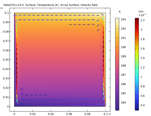
In the Model Builder window, expand the Results > Temperature and Fluid Flow (nitf1) node, then click Fluid Flow.
|
|
2
|
|
3
|
|
4
|
|
1
|
|
2
|
|
1
|
|
2
|
|
3
|
|
4
|
|
5
|
Click
|
|
1
|
|
2
|
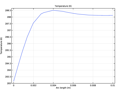
In the Settings window for 1D Plot Group, type Temperature at Boundary Layer in the Label text field.
|
|
3
|
|
4
|
|
1
|
|
2
|
In the Settings window for Line Graph, click Replace Expression in the upper-right corner of the y-Axis Data section. From the menu, choose Component 1 (comp1) > Heat Transfer in Fluids > Temperature > T - Temperature - K.
|
|
3
|
|
1
|
|
2
|
|
3
|
|
4
|
|
1
|
|
2
|
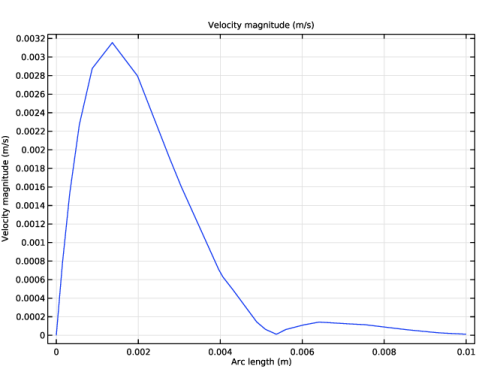
In the Settings window for Line Graph, click Replace Expression in the upper-right corner of the y-Axis Data section. From the menu, choose Component 1 (comp1) > Laminar Flow > Velocity and pressure > spf.U - Velocity magnitude - m/s.
|
|
3
|
|
1
|
|
2
|
Go to the Add Physics window.
|
|
3
|
|
4
|
Find the Physics interfaces in study subsection. In the table, clear the Solve checkbox for Study 1.
|
|
5
|
Click the Add to Component 2 button in the window toolbar.
|
|
6
|
|
1
|
|
2
|
Go to the Add Study window.
|
|
3
|
|
4
|
Find the Physics interfaces in study subsection. In the table, clear the Solve checkboxes for Laminar Flow (spf) and Heat Transfer in Fluids (ht).
|
|
5
|
Find the Multiphysics couplings in study subsection. In the table, clear the Solve checkbox for Nonisothermal Flow 1 (nitf1).
|
|
6
|
Click the Add Study button in the window toolbar.
|
|
7
|
|
1
|
|
2
|
|
3
|
|
4
|
|
5
|
|
6
|
|
1
|
|
2
|
Go to the Add Material window.
|
|
3
|
|
4
|
Click the Add to Component button in the window toolbar.
|
|
5
|
|
1
|
|
2
|
|
3
|
Select the Include gravity checkbox.
|
|
1
|
|
1
|
|
1
|
|
2
|
|
3
|
|
1
|
In the Model Builder window, under Component 2 (comp2) > Heat Transfer in Fluids 2 (ht2) click Initial Values 1.
|
|
2
|
|
3
|
|
1
|
|
3
|
|
4
|
|
1
|
|
3
|
|
4
|
|
1
|
|
1
|
|
2
|
|
3
|
Find the Pseudo time stepping subsection. From the Use pseudo time stepping for stationary equation form list, choose Off.
|
|
1
|
In the Model Builder window, under Component 2 (comp2) > Multiphysics click Nonisothermal Flow 2 (nitf2).
|
|
2
|
|
3
|
Select the Boussinesq approximation checkbox.
|
|
1
|
|
1
|
|
3
|
|
4
|
|
5
|
|
6
|
|
7
|
Select the Symmetric distribution checkbox.
|
|
8
|
|
1
|
|
2
|
|
3
|
|
4
|
|
5
|
|
6
|
Select the Reverse direction checkbox.
|
|
1
|
|
3
|
|
4
|
|
5
|
|
6
|
|
7
|
Click
|
|
1
|
|
2
|
|
3
|
|
1
|
|
2
|
|
3
|
|
4
|
Click
|
|
1
|
|
2
|
|
3
|
Select the Auxiliary sweep checkbox.
|
|
4
|
Click
|
|
1
|
|
2
|
|
4
|
Click to expand the Mesh Selection section. In the table, enter the following settings:
|
|
5
|
Click to expand the Values of Dependent Variables section. Find the Initial values of variables solved for subsection. From the Settings list, choose User controlled.
|
|
6
|
|
7
|
|
8
|
|
1
|
|
2
|
|
3
|
|
4
|
|
1
|
|
2
|
In the Model Builder window, expand the Study 2 > Solver Configurations > Solution 2 (sol2) > Stationary Solver 1 node, then click Fully Coupled 1.
|
|
3
|
|
4
|
|
5
|
In the Model Builder window, expand the Study 2 > Solver Configurations > Solution 2 (sol2) > Stationary Solver 2 node, then click Fully Coupled 1.
|
|
6
|
|
7
|
|
8
|
|
9
|
In the Model Builder window, expand the Study 2 > Solver Configurations > Solution 2 (sol2) > Stationary Solver 2 > AMG, nonisothermal flow (nitf2) node, then click Multigrid 1.
|
|
10
|
|
11
|
|
12
|
|
1
|
|
2
|
|
3
|
|
1
|
|
2
|
|
3
|
|
4
|
|
1
|
|
2
|
|
3
|
|
4
|
|
1
|
In the Model Builder window, expand the Results > Temperature and Fluid Flow (nitf2) node, then click Temperature and Fluid Flow (nitf2).
|
|
2
|
|
3
|
|
1
|
|
2
|
|
3
|
|
4
|
|
5
|
|
1
|
|
2
|
|
3
|
|
1
|
|
2
|
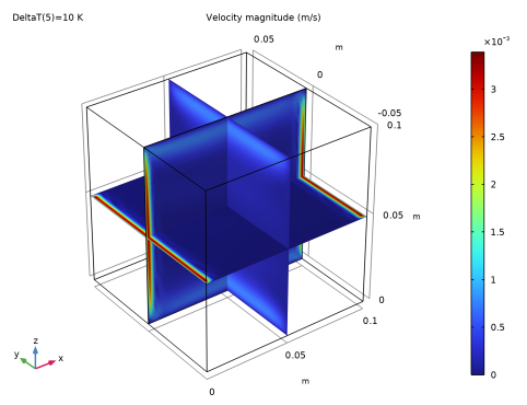
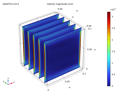
In the Settings window for Slice, click Replace Expression in the upper-right corner of the Expression section. From the menu, choose Component 2 (comp2) > Laminar Flow 2 > Velocity and pressure > spf2.U - Velocity magnitude - m/s.
|
|
3
|
|
4
|
|
1
|
|
2
|
|
3
|
|
1
|
|
2
|
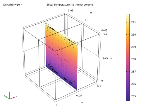
In the Settings window for Slice, click Replace Expression in the upper-right corner of the Expression section. From the menu, choose Component 2 (comp2) > Heat Transfer in Fluids 2 > Temperature > T2 - Temperature - K.
|
|
3
|
|
4
|
|
5
|
|
1
|
|
2
|
|
3
|
|
4
|
Locate the Arrow Positioning section. Find the x grid points subsection. In the Points text field, type 1.
|
|
5
|
|
6
|
|
7
|
|
8
|
|
1
|
|
2
|
|
3
|
|
4
|
|
1
|
|
2
|
|
3
|
|
4
|