PDF

Radiative Heat Transfer in a Utility Boiler
Introduction
In recent years, many studies have been conducted in the field of performance optimization of large power plant boilers. The main aims have been to extend the lifetime, increase the thermal efficiency, and reduce the pollutant emissions of the boilers. A good furnace design is the most important part in the energy conversion process in the boilers. A furnace is where the fuel is burnt and the chemical energy is converted into heat to be transferred into the water walls of steam boilers. The temperatures in fuel furnaces are high enough that the radiation becomes the most important mechanism in heat transfer. Due to complexity of the radiation mechanism and its dependence on the enclosure’s geometry, there is no analytical solution except for very simple problems. This fact along with expensive experimental modeling leads researchers to develop numerical models for analyzing these enclosures. Three of the most attractive methods, as far as accuracy and computational requirement are concerned, are the discrete transfer, the discrete ordinates and the finite-volume methods.
Note: Solving this application requires approximately 5 GB of memory.
Model Definition
Of practical relevance is the radiative heat transfer in furnaces containing obstacles, such as protrusions and obstructions. In some applications, the thickness of the obstacles is very small as it occurs in utility boilers, where panels are often hanged in the radiation chamber.
In order to reduce the mesh (and then the computational cost), these obstructions are modeled as baffles (zero thickness). This study handles zero thickness obstacles containing an emitting-absorbing medium.
A three-dimensional enclosure resembling the combustion chamber of a utility boiler is modeled. The study takes advantage of symmetries to model only one half of the combustion chamber, thereby reducing model size and computational costs. The enclosure contains three baffles, as shown in Figure 1, which simulates the panels of superheaters suspended at the top of the combustion chamber.
Figure 1: Half of the utility boiler with obstructions.
In this example, the S4 discrete ordinates method was employed for predicting the heat flux on the side walls of enclosures and incident radiation distribution within the furnace. It results in a set of 24 discrete directions to represent radiative intensity transport.
The main assumption is using an existing uniform temperature and properties within the volume and surface zones, as proposed in Ref. 1. The temperature and emissivity of the boundaries, including the surface of the baffles, are taken as 800 K and 0.65, respectively, except at x = 10 m and for 22  z ≤ 30 m, where the temperature was set equal to 1200 K and a blackbody surface is assumed. An emitting-absorbing medium is assumed, with the following distribution of temperature and absorption coefficient:
z 5
5 < z 10
10 < z 20
20 < z 30
Thermal Analysis
The discrete-ordinates method (DOM) relies on the discrete representation of the directional dependence of the radiation intensity. The radiative transfer equation (RTE) is solved for a set of discrete directions, si, which span the total solid angle range of 4π around a point in space.
The RTE for this type of configuration can be written as:
where
I(rs) is the radiative intensity at a given position r, following s direction
T is the temperature
κ, β, σs are absorption, extinction, and scattering coefficients, respectively
Ib(T) is the blackbody radiative intensity
ϕ(rs′, s) is the scattering function. ϕ(rs′, s) = 1 + a1μ0 and μ0 = s′ ⋅ s is the cosine of the scattering angle.
The boundary intensities in the furnace walls are given physically by the effective emitted intensity plus reflected incident intensities into a respective direction.
where
εw is the surface emissivity, which is in the range [01]
ρd = 1 − εw is the diffusive reflectivity
  n is the outward normal vector
qout is the heat flux striking the wall:
The above equations can be discretized in Cartesian coordinates for monochromatic or gray radiation as
The Sn approximation of the RTE in the m direction can be expressed as
For a discrete direction, si, the values of si1, si2, and si3 define the direction cosines of si obeying the condition si12 + si22 + si32 = 1. The j index in the above equation denotes the direction of incoming radiation contributing to the direction si.
For a diffuse reflecting surface on a wall boundary, the boundary condition equation is transformed as
Results and Discussion
Figure 2 and Figure 3 show the predicted incident radiation surface plots. The maximum incident radiation occurs at the level where the temperature and absorbing coefficient of the medium are the highest (that is, at the boiler’s burner level).
Figure 2: Incident radiation.
Figure 3: Incident radiation on the front of the boiler (W/m2).
The predicted outgoing heat flux is shown in Figure 4 and is in good agreement with published data (Ref. 1).
Figure 4: Outgoing heat flux on walls of the boiler (W/m2).
Reference
1. P.J. Coelho, J.M. Goncalves, and M.G. Carvalho, “Modelling of Radiative Heat Transfer in Enclosures with Obstacles,” Int’l J. Heat and Mass Transfer, vol. 41, no. 4–5, pp. 745–756, 1998.
Application Library path: Heat_Transfer_Module/Thermal_Radiation/boiler
Modeling Instructions
From the File menu, choose New.
New
In the New window, click  Model Wizard.
Model Wizard
1
In the Model Wizard window, click  3D.
2
In the Select Physics tree, select Heat Transfer > Radiation > Radiation in Participating Media (rpm).
3
Click Add.
4
Click  Study.
5
In the Select Study tree, select General Studies > Stationary.
6
Global Definitions
Parameters 1
1
In the Model Builder window, under Global Definitions click Parameters 1.
2
In the Settings window for Parameters, locate the Parameters section.
3
Piecewise 1 (pw1)
1
In the Home toolbar, click  Functions and choose Global > Piecewise.
2
In the Settings window for Piecewise, type T in the Function name text field.
3
Locate the Definition section. In the Argument text field, type z.
4
Find the Intervals subsection. In the table, enter the following settings:
5
Locate the Units section. In the Arguments text field, type m.
6
In the Function text field, type K.
Piecewise 2 (pw2)
1
In the Home toolbar, click  Functions and choose Global > Piecewise.
2
In the Settings window for Piecewise, type absC in the Function name text field.
3
Locate the Definition section. In the Argument text field, type z.
4
Find the Intervals subsection. In the table, enter the following settings:
5
Locate the Units section. In the Arguments text field, type m.
6
In the Function text field, type 1/m.
Geometry 1
Work Plane 1 (wp1)
1
In the Geometry toolbar, click  Work Plane.
2
In the Settings window for Work Plane, locate the Plane Definition section.
3
From the Plane list, choose xz-plane.
4
Click  Go to Plane Geometry.
Work Plane 1 (wp1) > Polygon 1 (pol1)
1
In the Work Plane toolbar, click  Polygon.
2
In the Settings window for Polygon, locate the Coordinates section.
3
From the Data source list, choose Vectors.
4
In the xw text field, type 0 0 0 10 10 10 10 8 8 10 10 10 10 6 6 4 4 0.
5
In the yw text field, type 4 30 30 30 30 22 22 20 20 18 18 4 4 0 0 0 0 4.
6
In the Work Plane toolbar, click  Build All.
Work Plane 1 (wp1) > Rectangle 1 (r1)
1
In the Work Plane toolbar, click  Rectangle.
2
In the Settings window for Rectangle, locate the Size and Shape section.
3
In the Width text field, type 4.
4
In the Height text field, type 10.
5
Locate the Position section. In the yw text field, type 20.
6
In the Work Plane toolbar, click  Build All.
Extrude 1 (ext1)
1
In the Model Builder window, right-click Geometry 1 and choose Extrude.
2
In the Settings window for Extrude, locate the Distances section.
3
4
In the Geometry toolbar, click  Build All.
5
Click the  Wireframe Rendering button in the Graphics toolbar.
6
Click the  Zoom Extents button in the Graphics toolbar.
The geometry should correspond to that in Figure 1.
Materials
Add a material to specify the absorption and scattering coefficients inside the boiler.
Chamber
1
In the Materials toolbar, click  Blank Material.
2
In the Settings window for Material, type Chamber in the Label text field.
3
Locate the Material Contents section. In the table, enter the following settings:
Analogously, specify the emissivity of the boiler walls using a material.
Walls
1
In the Materials toolbar, click  Blank Material.
2
In the Settings window for Material, type Walls in the Label text field.
3
Locate the Geometric Entity Selection section. From the Geometric entity level list, choose Boundary.
4
From the Selection list, choose All boundaries.
5
Locate the Material Contents section. In the table, enter the following settings:
Radiation in Participating Media (rpm)
By default, the Discrete ordinates method is S4, which corresponds to 24 discrete angular directions.
Participating Medium 1
1
In the Model Builder window, under Component 1 (comp1) > Radiation in Participating Media (rpm) click Participating Medium 1.
2
In the Settings window for Participating Medium, locate the Model Input section.
3
In the T text field, type T(z).
Initial Values 1
1
In the Model Builder window, click Initial Values 1.
2
In the Settings window for Initial Values, locate the Initial Values section.
3
In the Tinit text field, type T(z).
Opaque Surface 1
1
In the Model Builder window, click Opaque Surface 1.
2
In the Settings window for Opaque Surface, locate the Model Input section.
3
In the T text field, type Tlow.
Opaque Surface 2
1
In the Physics toolbar, click  Boundaries and choose Opaque Surface.
2
For more convenience in selecting these boundaries, you can click the Paste Selection button and paste the above numbers.
3
In the Settings window for Opaque Surface, locate the Model Input section.
4
In the T text field, type Thot.
5
Locate the Surface Radiative Properties section. From the Surface type list, choose Black surface.
Opaque Surface 3
1
In the Physics toolbar, click  Boundaries and choose Opaque Surface.
2
3
In the Settings window for Opaque Surface, locate the Model Input section.
4
In the T text field, type Tlow.
Opaque Surface 4
1
In the Physics toolbar, click  Boundaries and choose Opaque Surface.
2
3
In the Settings window for Opaque Surface, locate the Model Input section.
4
In the T text field, type Tlow.
5
Locate the Surface Radiative Properties section. Select the Define properties on each side checkbox.
6
Find the Emissivity subsection. From the εu list, choose User defined.
Symmetry 1
1
In the Physics toolbar, click  Boundaries and choose Symmetry.
2
Mesh 1
Mapped 1
1
In the Mesh toolbar, click  More Generators and choose Mapped.
2
3
In the Settings window for Mapped, click  Build Selected.
Free Quad 1
1
In the Mesh toolbar, click  More Generators and choose Free Quad.
2
3
In the Settings window for Free Quad, click  Build Selected.
Swept 1
In the Mesh toolbar, click  Swept.
Size
1
In the Model Builder window, click Size.
2
In the Settings window for Size, locate the Element Size section.
3
From the Predefined list, choose Extra fine.
4
In the Model Builder window, right-click Mesh 1 and choose Build All.
Study 1
In the Study toolbar, click  Compute.
Results
Incident Radiation (rpm)
The default plot group shows the Incident Radiation multislice plot. Follow the instructions below to replace the multislice plot for Incident Radiation by a contour plot.
Multislice 1
1
In the Model Builder window, expand the Incident Radiation (rpm) node.
2
Right-click Multislice 1 and choose Delete.
3
Click Yes to confirm.
Incident Radiation (rpm)
In the Model Builder window, under Results click Incident Radiation (rpm).
Contour 1
1
In the Incident Radiation (rpm) toolbar, click  Contour.
2
In the Settings window for Contour, locate the Levels section.
3
From the Entry method list, choose Levels.
4
In the Levels text field, type range(0,1e5,21e5).
5
Locate the Coloring and Style section. From the Contour type list, choose Filled.
6
Click to expand the Quality section. From the Evaluation settings list, choose Manual.
7
From the Smoothing list, choose None.
8
In the Incident Radiation (rpm) toolbar, click  Plot.
9
Click the  Zoom Extents button in the Graphics toolbar to get the results shown in Figure 2.
10
Click the  Go to YZ View button in the Graphics toolbar to reproduce the results in Figure 3.
In Figure 4, the outgoing radiative heat flux is plotted for the full 3D geometry. Even if only one half of the utility boiler is modeled the solution can be mirrored to obtain a full 3D view of the results. To do so, follow the steps below:
Mirror 3D 1
1
In the Model Builder window, expand the Results > Datasets node.
2
Right-click Results > Datasets and choose More 3D Datasets > Mirror 3D.
3
In the Settings window for Mirror 3D, locate the Plane Data section.
4
From the Plane list, choose XZ-planes.
5
In the Y-coordinate text field, type -6.
6
Outgoing Radiative Heat Flux (rpm)
1
In the Results toolbar, click  3D Plot Group.
2
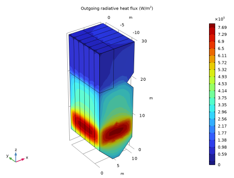
In the Settings window for 3D Plot Group, type Outgoing Radiative Heat Flux (rpm) in the Label text field.
3
Locate the Data section. From the Dataset list, choose Mirror 3D 1.
Contour 1
1
In the Outgoing Radiative Heat Flux (rpm) toolbar, click  Contour.
2
In the Settings window for Contour, click Replace Expression in the upper-right corner of the Expression section. From the menu, choose Component 1 (comp1) > Radiation in Participating Media > Boundary fluxes > rpm.qr_out - Outgoing radiative heat flux - W/m².
3
Locate the Coloring and Style section. From the Contour type list, choose Filled.
4
Locate the Quality section. From the Evaluation settings list, choose Manual.
5
From the Smoothing list, choose None.
Outgoing Radiative Heat Flux (rpm)
Click the  Go to Default View button in the Graphics toolbar to obtain Figure 4.