PDF

Grain Separation Using Vibrating Sieves
Introduction
Grain separation is an important process wherein a mixture of various species of grains are separated to isolate the grains based on their desired characteristics. It is used in numerous industries including agriculture, mining, food processing, and milling. A common and simple method of grain separation that utilizes gravity is to pass the grains through a sieve with holes so that the grains smaller than the holes can pass through, while the sieve filters out the larger grains. A series of sieves of different sizes can be strategically constructed to achieve multiple levels of separation based on grain size and shape. The separation speed can often be enhanced by vibrating the sieves, which has the effect of keeping the grains in constant motion, thus increasing the chances of a grain encountering a hole.
This example uses the Granular Flow interface to model the separation of a mixture containing grains of three sizes as they pass through two vibrating sieves with holes of different sizes. The separation efficiency of the machine is then quantified.
Model Definition
The geometry of the model consists of a rectangular box of dimensions 40 cm-by-100 cm-by-40 cm. The top surface has a rectangular inlet surface through which grains of diameters 10, 20, and 30 mm enter the box. Two sieves are located at heights of 10 cm and 20 cm from the bottom surface. The top sieve has a rectangular array of square-shaped holes of length 25 mm. The bottom sieve similarly has holes of length 12.5 mm. The entire box is then tilted so that it has an inclination angle of 5 degrees. This tilt helps the grains move away from the inlet surface through gravity, thus enhancing the chances of the grains encountering the holes, and also keeps the separated grains moving. The geometry is presented in Figure 1 which shows the domain being divided into three compartments by the two sieves.
The grains are continuously released through the inlet for a period of 1.0 s at a frequency of 0.1 s. At each release time, a total of 500 grains are released such that the three types of grains have the same mass fractions. Both the sieves are vibrated with an amplitude of 5 mm and a frequency of 11 Hz. The vibrations are confined to the plane defined by the sieve. The mixture of grains pass through the two vibrating sieves which are designed such that the top sieve filters out the largest grains, while the bottom sieve filters out the medium-sized grains. The model is simulated for a total of 10 s.
Since, an ideal operation of the process filters out the three types of grains completely into the three compartments, we define a separation efficiency parameter to quantify the quality of the process. The separation efficiency is defined for each type of grain as the ratio of the total mass of the grains (belonging to that grain type) in its ideal compartment divided by the total mass of that grain type in the domain.
Figure 1: Model geometry.
Notes on the COMSOL Implementation
The model is solved using a single Time Dependent study step. The three types of grains are released into the domain using the Inlet feature. The vibration of the sieves is controlled by the Wall Movement settings in the Wall feature where a prescribed displacement is used to specify the rigid body motion of the sieves. This displacement is explicitly calculated by defining variables in the Variables node.
In order to evaluate the compartment that a grain belongs to at any given time, it is enough to measure the normal distance from the bottom stationary surface of the domain. When the entire domain is tilted as is the case in this model, this distance calculation can be simplified by defining a new orthogonal coordinate system whose xy-plane is oriented along the bottom surface. In this model, this is achieved by adding a System from Geometry node under the Boundary System node. The z coordinate in this new coordinate system can be used to identify the compartment a grain belongs to.
The maximum allowed time step taken by the Time-Dependent Solver in Granular Flow is often limited by the collision time scales of the grain-grain and grain-wall interactions. The collision time scales are often strongly dependent on the material properties such as density and Young’s modulus with stiffer grains generally exhibiting smaller collision times, thus requiring even smaller time steps. In many instances however, the stiffness of the grains and walls have a very limited effect on the bulk behavior of granular materials, and the materials can thus be made artificially less stiff in order to speed up the simulations.
Results and Discussion
The grain positions at the end of the 10 s is shown in Figure 2. The grains are colored based on their diameters. It can be seen that the top sieve completely filters out the largest (red) grains since they are too big to pass through its holes. Similarly, the bottom sieve has holes that are too small for the medium-sized (green) grains to pass through and therefore only the smallest grains are found in the bottom compartment. However, the separation is not ideal as some of the small grains can be seen in all the compartments, and some of the medium-sized grains can also be seen in the top compartment.
Figure 2: Grains of three different sizes being separated using vibrating sieves. The grains are colored by their diameters in mm.
Figure 3 shows the overall number of the small grains in each compartment (bin) as a function of time. The number of small grains in the top bin rises sharply in the beginning as grains are release into the domain. However, as time progresses, this number slowly decreases as these grains filter down into the middle and bottom bins. The number of small grains in the bottom bin rises steadily until most of the grains have reached this bin, while the number in the middle bin rises slowly and then quickly falls as expected.
Figure 3: The distribution of the small grains across the three bins.
Figure 4: The separation efficiency of the sieves as a function of time.
Finally, the separation efficiency for all three grain types are shown as a function of time in Figure 4. The efficiency curves for the small and medium grains increase steadily as a function of time and saturates at values between 0.95 and 1.0, while the efficiency curves for the large grains exhibit a noisy behavior up to 1.0 s. This is due to new grains being released at discrete time intervals. After 1 s however, the separation efficiency of the large grains quickly approaches 1.0 as they are completely filtered out by the top sieve.
Application Library path: Granular_Flow_Module/Mixing_and_Separation/vibrating_sieves
Modeling Instructions
From the Main Toolbar menu, choose New.
New
In the New window, click  Model Wizard.
Model Wizard
1
In the Model Wizard window, click  3D.
2
In the Select Physics tree, select Fluid Flow > Granular Flow (gran).
3
Click Add.
4
Click  Study.
5
In the Select Study tree, select General Studies > Time Dependent.
6
Global Definitions
Parameters 1
1
In the Model Builder window, under Global Definitions click Parameters 1.
2
In the Settings window for Parameters, locate the Parameters section.
3
Click  Load from File.
4
Geometry 1
Block 1 (blk1)
1
In the Geometry toolbar, click  Block.
2
In the Settings window for Block, locate the Size and Shape section.
3
In the Width text field, type Lx.
4
In the Depth text field, type Ly.
5
In the Height text field, type Lz.
Work Plane 1 (wp1)
1
In the Geometry toolbar, click  Work Plane.
2
In the Settings window for Work Plane, locate the Plane Definition section.
3
In the z-coordinate text field, type Lz.
4
Click  Build Selected.
Work Plane 1 (wp1) > Plane Geometry
In the Model Builder window, click Plane Geometry.
Work Plane 1 (wp1) > Rectangle 1 (r1)
1
In the Work Plane toolbar, click  Rectangle.
2
In the Settings window for Rectangle, locate the Size and Shape section.
3
In the Width text field, type Lx.
4
In the Height text field, type inlet_width.
5
Locate the Position section. In the yw text field, type Ly-inlet_width.
6
Click  Build Selected.
Work Plane 2 (wp2)
1
In the Model Builder window, right-click Geometry 1 and choose Work Plane.
2
In the Settings window for Work Plane, locate the Plane Definition section.
3
In the z-coordinate text field, type Lz/4.
Work Plane 2 (wp2) > Plane Geometry
In the Model Builder window, click Plane Geometry.
Work Plane 2 (wp2) > Rectangle 1 (r1)
1
In the Work Plane toolbar, click  Rectangle.
2
In the Settings window for Rectangle, locate the Size and Shape section.
3
In the Width text field, type Lx.
4
In the Height text field, type Ly.
Work Plane 2 (wp2) > Square 1 (sq1)
1
In the Work Plane toolbar, click  Square.
2
In the Settings window for Square, locate the Size section.
3
In the Side length text field, type hole_width.
4
Locate the Position section. In the xw text field, type hole_width.
5
In the yw text field, type hole_width.
6
Click  Build Selected.
Work Plane 2 (wp2) > Array 1 (arr1)
1
In the Work Plane toolbar, click  Transforms and choose Array.
2
3
In the Settings window for Array, locate the Size section.
4
In the xw size text field, type floor(0.99*Lx/hole_width/2).
5
In the yw size text field, type floor(0.99*Ly/hole_width/2).
6
Locate the Displacement section. In the xw text field, type 2*hole_width.
7
In the yw text field, type 2*hole_width.
8
Click  Build Selected.
Work Plane 2 (wp2) > Difference 1 (dif1)
1
In the Work Plane toolbar, click  Booleans and Partitions and choose Difference.
2
3
In the Settings window for Difference, locate the Difference section.
4
From the Objects to subtract list, choose All objects.
5
Click to select the  Activate Selection toggle button for Objects to subtract.
6
7
Click the  Remove from Selection button for Objects to subtract.
8
Click  Build Selected.
Work Plane 3 (wp3)
1
In the Model Builder window, under Component 1 (comp1) > Geometry 1 right-click Work Plane 2 (wp2) and choose Duplicate.
2
In the Model Builder window, click Work Plane 3 (wp3).
3
In the Settings window for Work Plane, locate the Plane Definition section.
4
In the z-coordinate text field, type Lz/2.
Work Plane 3 (wp3) > Square 1 (sq1)
1
In the Model Builder window, expand the Component 1 (comp1) > Geometry 1 > Work Plane 3 (wp3) > Plane Geometry node, then click Square 1 (sq1).
2
In the Settings window for Square, locate the Size section.
3
In the Side length text field, type hole_width*2.
4
Locate the Position section. In the xw text field, type hole_width*2.
5
In the yw text field, type hole_width*2.
6
Click  Build Selected.
Work Plane 3 (wp3) > Array 1 (arr1)
1
In the Model Builder window, click Array 1 (arr1).
2
In the Settings window for Array, locate the Size section.
3
In the xw size text field, type floor(0.99*Lx/hole_width/4).
4
In the yw size text field, type floor(0.99*Ly/hole_width/4).
5
Locate the Displacement section. In the xw text field, type 4*hole_width.
6
In the yw text field, type 4*hole_width.
7
Click  Build Selected.
Rotate 1 (rot1)
1
In the Model Builder window, right-click Geometry 1 and choose Transforms > Rotate.
2
In the Settings window for Rotate, locate the Input section.
3
From the Input objects list, choose All objects.
4
Locate the Rotation section. From the Axis type list, choose x-axis.
5
In the Angle text field, type theta.
6
Click  Build Selected.
Work Plane 4 (wp4)
1
In the Geometry toolbar, click  Work Plane.
2
In the Settings window for Work Plane, locate the Plane Definition section.
3
From the Plane type list, choose Face parallel.
4
On the object rot1(1), select Boundary 1 only.
5
Click  Build All Objects.
6
Click the  Show Grid button in the Graphics toolbar.
7
Click the  Transparency button in the Graphics toolbar.
8
Click the  Go to Default View button in the Graphics toolbar. The geometry should look like Figure 1.
9
In the Definitions toolbar, click  Coordinate Systems and choose System from Geometry.
Definitions
System from Geometry 2 (sys2)
1
In the Settings window for System from Geometry, locate the System from Geometry section.
2
From the Work plane list, choose Work Plane 4 (wp4).
Variables 1
1
In the Definitions toolbar, click  Local Variables.
2
In the Settings window for Variables, locate the Variables section.
3
Materials
Grains
1
In the Materials toolbar, click  Blank Material.
2
In the Settings window for Material, type Grains in the Label text field.
3
Click to expand the Material Properties section. In the Material properties tree, select Basic Properties > Density.
4
Click  Add to Material.
5
In the Material properties tree, select Basic Properties > Poisson’s Ratio.
6
Click  Add to Material.
7
In the Material properties tree, select Basic Properties > Young’s Modulus.
8
Click  Add to Material.
9
Locate the Material Contents section. In the table, enter the following settings:
Walls
1
In the Materials toolbar, click  Blank Material.
2
In the Settings window for Material, type Walls in the Label text field.
3
Locate the Geometric Entity Selection section. From the Geometric entity level list, choose Boundary.
4
From the Selection list, choose All boundaries.
5
Locate the Material Contents section. In the table, enter the following settings:
Granular Flow (gran)
Small Grains
1
In the Model Builder window, under Component 1 (comp1) > Granular Flow (gran) click Grain Properties 1.
2
In the Settings window for Grain Properties, type Small Grains in the Label text field.
3
Locate the Granular Material Properties section. From the Granular material list, choose Grains (mat1).
4
Locate the Size section. In the dg text field, type dg.
Medium Grains
1
In the Physics toolbar, click  Global and choose Grain Properties.
2
In the Settings window for Grain Properties, type Medium Grains in the Label text field.
3
Locate the Granular Material Properties section. From the Granular material list, choose Grains (mat1).
4
Locate the Size section. In the dg text field, type 2*dg.
Large Grains
1
Right-click Medium Grains and choose Duplicate.
2
In the Settings window for Grain Properties, type Large Grains in the Label text field.
3
Locate the Size section. In the dg text field, type 3*dg.
Contact Between Grains 1
1
In the Model Builder window, click Contact Between Grains 1.
2
In the Settings window for Contact Between Grains, locate the Contact Properties section.
3
In the en text field, type e.
4
In the et text field, type e.
5
In the μs text field, type 0.5.
6
In the μr text field, type 0.01.
7
In the μtw text field, type 0.01.
Contact with Walls 1
1
In the Model Builder window, click Contact with Walls 1.
2
In the Settings window for Contact with Walls, locate the Contact Properties section.
3
In the en text field, type e.
4
In the et text field, type e.
5
In the μs text field, type 0.5.
6
In the μr text field, type 0.01.
7
In the μtw text field, type 0.01.
Inlet 1
1
In the Physics toolbar, click  Boundaries and choose Inlet.
2
3
In the Settings window for Inlet, locate the Release Times section.
4
In the Release times text field, type range(0,0.1,1).
5
Locate the Released Grain Properties section. From the Distribution of released grain properties list, choose Mass fraction.
6
In the N text field, type 500.
7
Vibrating Sieves
1
In the Physics toolbar, click  Boundaries and choose Wall.
2
In the Settings window for Wall, type Vibrating Sieves in the Label text field.
3
4
Locate the Wall Movement section. From the Wall motion list, choose Translation.
5
Specify the dx vector as
Study 1
Step 1: Time Dependent
1
In the Model Builder window, under Study 1 click Step 1: Time Dependent.
2
In the Settings window for Time Dependent, locate the Study Settings section.
3
In the Output times text field, type range(0,0.05,10).
4
In the Study toolbar, click  Compute.
Results
Grain Positions (gran)
In the Model Builder window, expand the Grain Positions (gran) node.
Color Expression 1
1
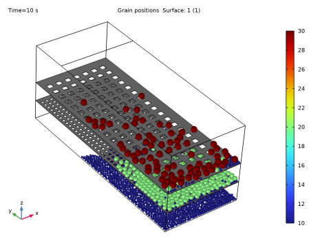
In the Model Builder window, expand the Results > Grain Positions (gran) > Grain Positions 1 node, then click Color Expression 1.
2
In the Settings window for Color Expression, locate the Expression section.
3
In the Expression text field, type gran.dg.
4
From the Unit list, choose mm.
5
Click the  Go to Default View button in the Graphics toolbar.
6
Click the  Transparency button in the Graphics toolbar.
7
In the Grain Positions (gran) toolbar, click  Plot. The grain positions at the end of the study should resemble Figure 2.
Animation 1
1
In the Grain Positions (gran) toolbar, click  Animation and choose Player.
2
In the Settings window for Animation, locate the Frames section.
3
From the Frame selection list, choose All.
4
Click the  Play button in the Graphics toolbar.
Distribution of small grains
1
In the Results toolbar, click  1D Plot Group.
2
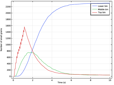
In the Settings window for 1D Plot Group, type Distribution of small grains in the Label text field.
3
Locate the Data section. From the Dataset list, choose Grain 1.
4
Locate the Plot Settings section.
5
Select the x-axis label checkbox. In the associated text field, type Time (s).
6
Select the y-axis label checkbox. In the associated text field, type Number of small grains.
Global 1
1
In the Distribution of small grains toolbar, click  Global.
2
In the Settings window for Global, locate the y-Axis Data section.
3
4
In the Distribution of small grains toolbar, click  Plot. The distribution of the small grains across the three bins as a function of time should resemble Figure 3.
Separation Efficiency
1
In the Results toolbar, click  1D Plot Group.
2
In the Settings window for 1D Plot Group, type Separation Efficiency in the Label text field.
3
Locate the Data section. From the Dataset list, choose Grain 1.
4
Locate the Plot Settings section.
5
Select the x-axis label checkbox. In the associated text field, type Time (s).
6
Select the y-axis label checkbox. In the associated text field, type Efficiency.
7
Locate the Legend section. From the Position list, choose Lower right.
Global 1
1
In the Separation Efficiency toolbar, click  Global.
2
In the Settings window for Global, locate the y-Axis Data section.
3
4
In the Separation Efficiency toolbar, click  Plot. The separation efficiency as a function of time should resemble Figure 4.