PDF

Screw Conveyor
Introduction
A screw conveyor is a mechanical device that is commonly used to move bulk granular materials. They can be used to transport the materials either horizontally or over an incline, which also allows for elevating the material. Additional specialized tasks such as heating, cooling, drying and mixing can also be incorporated along with the transport process. Screw conveyors are widely used across various industries including food processing, pharmaceuticals, chemical industries, agriculture, cosmetics, and plastics.
A screw conveyor typically consists of a U-shaped trough or a tube with a rotating central shaft along its length. The central shaft contains helical screw that is rotated about its axis. The amount of material transported and its speed is affected by several factors including the material and contact properties of the grains and the walls, filling level of the trough, and rotational speed. The mass-flow rate is often proportional to the rotational speed.
This example uses the Granular Flow interface to model the transport of grains using a screw conveyor operated at a constant rotational speed. This model also shows the use of a Bounding Box feature to avoid scenarios that may adversely affect the performance of the Granular Flow interface. The mass-flow rate through the conveyor is evaluated using a Model Method.
Model Definition
The geometry consists of a cylindrical tube with a casing radius of 20.4 cm and a length of 1.3 m. A central shaft of radius 10 cm runs through the length of the tube. The central shaft has helical screw blades attached to it with a pitch of 20 cm and a gap of 4 mm between the blade and the tube. The overall length of the shaft is such that there are six turns of the helix. The tube and the screw are rotated to have an inclination of 10 degrees. The grains enter the tube via conical hopper and exit via a circular outlet at the other end of the tube. The geometry is presented in Figure 1.
The grains have a density of 4200 kg/m3 and a diameter of 10 mm. The grains are released in ten batches of 2500 grains each with an interval of 0.5 s. The screw is rotated at a constant angular speed of 120 rpm. The transport of the grains is simulated for a total of 20 s. The mass-flow rate through the screw conveyor is measured by evaluating the overall mass of the grains that pass through an imaginary plane in the middle of the tube.
Figure 1: Model geometry.
Notes About the COMSOL Implementation
The model is solved using a single Time Dependent study step. The grains are released into the conical hopper using the Release feature. The rotation of the screw is controlled by the Wall Movement settings in the Wall feature. The grains can pass through the interior boundaries and out of the tube using an Outlet feature. The grains exiting the tube can continue moving away from the trough, which can adversely affect the performance of the Granular Flow interface.
The maximum allowed time step taken by the Time-Dependent Solver in Granular Flow is often limited by the collision time scales of the grain-grain and grain-wall interactions. The collision time scales are often strongly dependent on the material properties such as density and Young’s modulus with stiffer grains generally exhibiting smaller collision times, thus requiring even smaller time steps. In many instances however, the stiffness of the grains and walls have a very limited effect on the bulk behavior of granular materials, and the materials can thus be made artificially less stiff in order to speed up the simulations.
A Bounding Box feature is used to remove such grains from the simulation. An user-defined variable is added to each grain to keep track of the grains that pass through an imaginary plane. The mass-flow rate can then be obtained by counting the overall mass of the grains that pass through the plane in a given time window divided by the length of the time window. This averaging of the time series data is achieved by adding and running a Model Method.
Note: Model methods can only be set up in the COMSOL Desktop environment on the Windows version of COMSOL Multiphysics.
Results and Discussion
A snapshot of the grain positions in the middle of the transport process is shown in Figure 2. The grains are colored based on their release time. The inclination and the gap between the blade and the tube causes some grains to be left behind at one end of the tube, while most of the grains are transported to the other end. There grain colors indicate that some amount of mixing occurs during the transport.
The forces experienced by the screw due to the grain impact is an important factor in the design and operation of a screw conveyor. Figure 3 shows the forces at the same instant of time as in Figure 2. It is clear that the maximum forces are experienced near the parts of the screw that is exposed to the largest number of grains. These forces can then be used to evaluate the power draw required to operate the conveyor and the wear rate of the screw blades.
Finally, Figure 4 presents the plot of the mass-flow rate as defined as the overall rate mass of the grains that transit an imaginary plane. Since the plane is located in the middle of the tube, the calculated flow rate is 0 in the beginning. It slowly rises until it reaches a peak of about 3.8 kg/s before it starts decreasing as the bulk of the grains pass through the plane. This peak could be interpreted as the overall mass-flow rate of the device when operated under similar conditions in a continuous configuration as opposed to the batch configuration used in this model.
Figure 2: Grain positions at the end of 10 seconds. The grains are colored by their release time.
Figure 3: Forces on the screw at the end of 10 seconds.
Figure 4: Mass-flow rate as a function of time.
Application Library path: Granular_Flow_Module/Transport/screw_conveyor
Modeling Instructions
From the Main Toolbar menu, choose New.
New
In the New window, click  Model Wizard.
Model Wizard
1
In the Model Wizard window, click  3D.
2
In the Select Physics tree, select Fluid Flow > Granular Flow (gran).
3
Click Add.
4
Click  Study.
5
In the Select Study tree, select General Studies > Time Dependent.
6
Geometry 1
1
In the Geometry toolbar, click Insert Sequence and choose Insert Sequence.
2
3
In the Geometry toolbar, click  Build All.
4
Click the  Transparency button in the Graphics toolbar.
5
Click the  Show Grid button in the Graphics toolbar.
6
Click the  Zoom Extents button in the Graphics toolbar. The geometry should look like Figure 1.
Global Definitions
Parameters 2
1
In the Home toolbar, click  Parameters and choose Add > Parameters.
2
In the Settings window for Parameters, locate the Parameters section.
3
Geometry 1
Work Plane 3 (wp3)
1
In the Geometry toolbar, click  Work Plane.
2
In the Settings window for Work Plane, locate the Plane Definition section.
3
From the Plane type list, choose Edge angle.
4
On the object del1, select Edge 3 only.
5
Click to select the  Activate Selection toggle button for Face adjacent to edge.
6
On the object del1, select Boundary 2 only.
7
Select the Reverse normal direction checkbox.
8
In the Definitions toolbar, click  Coordinate Systems and choose System from Geometry.
Definitions
System from Geometry 2 (sys2)
1
In the Settings window for System from Geometry, locate the System from Geometry section.
2
From the Work plane list, choose Work Plane 3 (wp3).
Variables 1
1
In the Home toolbar, click  Variables and choose Local Variables.
2
In the Settings window for Variables, locate the Variables section.
3
Materials
Grains
1
In the Materials toolbar, click  Blank Material.
2
In the Settings window for Material, type Grains in the Label text field.
3
Click to expand the Material Properties section. In the Material properties tree, select Basic Properties > Density.
4
Click  Add to Material.
5
In the Material properties tree, select Basic Properties > Poisson’s Ratio.
6
Click  Add to Material.
7
In the Material properties tree, select Basic Properties > Young’s Modulus.
8
Click  Add to Material.
9
Locate the Material Contents section. In the table, enter the following settings:
Walls
1
In the Materials toolbar, click  Blank Material.
2
In the Settings window for Material, type Walls in the Label text field.
3
Locate the Geometric Entity Selection section. From the Geometric entity level list, choose Boundary.
4
From the Selection list, choose All boundaries.
5
Locate the Material Contents section. In the table, enter the following settings:
Granular Flow (gran)
Grain Properties 1
1
In the Model Builder window, under Component 1 (comp1) > Granular Flow (gran) click Grain Properties 1.
2
In the Settings window for Grain Properties, locate the Granular Material Properties section.
3
From the Granular material list, choose Grains (mat1).
4
Locate the Size section. In the dg text field, type dg.
Release 1
1
In the Physics toolbar, click  Domains and choose Release.
2
3
In the Settings window for Release, locate the Release Times section.
4
In the Release times text field, type range(0,0.5,4.5).
5
Locate the Released Grain Properties section. In the table, enter the following settings:
Screw
1
In the Physics toolbar, click  Boundaries and choose Wall.
2
In the Settings window for Wall, type Screw in the Label text field.
3
Locate the Boundary Selection section. From the Selection list, choose Screw.
4
Locate the Wall Movement section. From the Wall motion list, choose Rotation.
5
In the ω text field, type om.
6
Specify the eax vector as
Force Accumulator 1
In the Physics toolbar, click  Attributes and choose Force Accumulator.
Contact Between Grains 1
1
In the Model Builder window, under Component 1 (comp1) > Granular Flow (gran) click Contact Between Grains 1.
2
In the Settings window for Contact Between Grains, locate the Contact Properties section.
3
In the en text field, type 0.8.
4
In the et text field, type 0.7.
5
In the μs text field, type 0.4.
6
In the μr text field, type 0.3.
7
In the μtw text field, type 0.25.
Contact with Walls 1
1
In the Model Builder window, click Contact with Walls 1.
2
In the Settings window for Contact with Walls, locate the Contact Properties section.
3
In the en text field, type 0.85.
4
In the et text field, type 0.76.
5
In the μs text field, type 0.5.
6
In the μr text field, type 0.2.
7
In the μtw text field, type 0.18.
Outlet 1
1
In the Physics toolbar, click  Boundaries and choose Outlet.
2
Bounding Box 1
1
In the Physics toolbar, click  Global and choose Bounding Box.
2
In the Settings window for Bounding Box, locate the Settings section.
3
From the Specify bounding box list, choose From geometry.
Study 1
Step 1: Time Dependent
1
In the Model Builder window, under Study 1 click Step 1: Time Dependent.
2
In the Settings window for Time Dependent, locate the Study Settings section.
3
In the Output times text field, type range(0,0.25,20).
4
In the Study toolbar, click  Compute.
Results
Grain Positions (gran)
1
In the Settings window for 3D Plot Group, locate the Data section.
2
From the Time (s) list, choose 10.
3
Click the  Transparency button in the Graphics toolbar.
4
Click the  Go to XZ View button in the Graphics toolbar.
5
Click the  Zoom Extents button in the Graphics toolbar.
6
In the Model Builder window, expand the Grain Positions (gran) node.
Color Expression 1
1
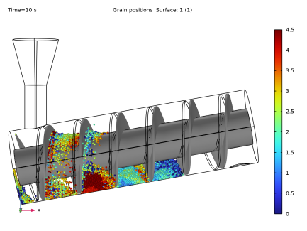
In the Model Builder window, expand the Results > Grain Positions (gran) > Grain Positions 1 node, then click Color Expression 1.
2
In the Settings window for Color Expression, locate the Expression section.
3
In the Expression text field, type gran.rti.
4
In the Grain Positions (gran) toolbar, click  Plot. The plot should look like Figure 2.
Forces on the screw
1
In the Results toolbar, click  3D Plot Group.
2
In the Settings window for 3D Plot Group, type Forces on the screw in the Label text field.
3
Locate the Data section. From the Dataset list, choose Grain 1.
4
From the Time (s) list, choose 10.
5
Locate the Plot Settings section. Clear the Plot dataset edges checkbox.
Surface 1
1
In the Forces on the screw toolbar, click  Surface.
2
In the Settings window for Surface, locate the Expression section.
3
In the Expression text field, type gran.wp2.facc1.wf.
4
Locate the Coloring and Style section. From the Color table list, choose PrismDark.
Deformation 1
1
In the Forces on the screw toolbar, click  Deformation.
2
In the Settings window for Deformation, locate the Expression section.
3
In the x-component text field, type comp1.gran.x-x.
4
In the y-component text field, type comp1.gran.y-y.
5
In the z-component text field, type comp1.gran.z-z.
6
Locate the Scale section.
7
Select the Scale factor checkbox. In the associated text field, type 1.0.
Surface 1
In the Model Builder window, click Surface 1.
Selection 1
1
In the Forces on the screw toolbar, click  Selection.
2
In the Settings window for Selection, locate the Selection section.
3
From the Selection list, choose Screw.
4
In the Forces on the screw toolbar, click  Plot. The plot should look like Figure 3.
Grain Positions
1
In the Forces on the screw toolbar, click  Animation and choose Player.
2
In the Settings window for Animation, type Grain Positions in the Label text field.
3
Locate the Scene section. From the Subject list, choose Grain Positions (gran).
4
Locate the Frames section. From the Frame selection list, choose All.
5
Click the  Play button in the Graphics toolbar. This plays the animation of the grains being transported by the screw conveyor.
Forces on the Screw
1
Right-click Grain Positions and choose Duplicate.
2
In the Settings window for Animation, type Forces on the Screw in the Label text field.
3
Locate the Scene section. From the Subject list, choose Forces on the screw.
4
Click the  Play button in the Graphics toolbar. This plays the animation of the forces on the screw conveyor resulting from the grain-wall contacts.
Application Builder
The mass flow rate can be computed using an Application Method. These may be added to an existing model via a Model Method using the Application Builder. Note that the Application Builder is only available in the Windows® version of the COMSOL Desktop. But once the Model Method is created, it can be run in both the Linux and Mac versions.
In the Home toolbar, click  Application Builder.
Methods
The code for the computing and plotting the mass flow rate can be simplified by using utility classes.
util1
1
In the Home toolbar, click  More Libraries and choose Utility Class.
2
In the Application Builder window, right-click util1 and choose Edit.
3
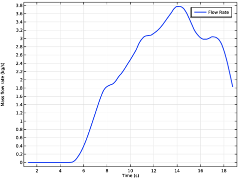
Copy the code for the utilities createGrainEval, createGridDataSets, updateDatsets, plotFlowRate and getPlotFeature and paste it into the Utility Class editor for util1.
// Create the Grain evaluations
 public static NumericalFeature createGrainEval(String tag, String data, String level, NumericalFeatureList numericalList) {
   NumericalFeature grn;
   if (numericalList.index(tag) == -1)
     grn = model.result().numerical().create(tag, "Grain");
   else
     grn = numericalList.get(tag);
   grn.setIndex("looplevelinput", level, 0);
   grn.set("data", data);
   return grn;
 }
 
 /* Create the interpolation functions and the grid data sets*/
 public static void createGridDataSets(String[] myTags, int num_steps, double[][] data) {
   FunctionFeatureList functionList = model.func();
   FunctionFeature functionFeature;
   
   for (int i = 0; i < myTags.length; i++) {
     if (functionList.index(myTags[i]) == -1) {
       functionFeature = functionList.create(myTags[i], "Interpolation");
       functionFeature.label(myTags[i]);
       with(functionFeature);
         set("funcname", myTags[i]);
         set("interp", "piecewisecubic");
         set("extrap", "const");
         set("defineprimfun", true);
       endwith();
     }
     else {
       functionFeature = functionList.get(myTags[i]);
     }
     
     with(functionFeature);
       set("table", new String[0][0]);
       for (int k = 0; k < num_steps; k++) {
         setIndex("table", data[k][0], k, 0);
         setIndex("table", data[k][i+1], k, 1);
       }
     endwith();
     
     String pmin = toString(data[0][0]);
     String pmax = toString(data[num_steps-1][0]);
     String[] params = {pmin, pmax, "out"};
     util1.updateDatsets(i, params, myTags);
   }
 }
 
 /** Create or update the grid datasets. */
 public static void updateDatsets(int i, String[] param,
                                  String[] tagList) {
   DatasetFeature dataFeature;
   if (model.result().dataset().index(tagList[i]) == -1) {
     dataFeature = model.result().dataset().create(tagList[i], "Grid1D");
     dataFeature.label(tagList[i]);
   }
   else {
     dataFeature = model.result().dataset().get(tagList[i]);
   }
   with(dataFeature);
     set("source", "function");
     set("function", tagList[i]);
     set("parmin1", param[0]);
     set("parmax1", param[1]);
     set("par1", param[2]);
   endwith();
 }
 
 /* Add the line plots for the flow rate */
 public static void plotFlowRate(String[] myList, String[] myTags)
 {
   // Create or get the plot group
   ResultFeature myPlot = util1.getPlotFeature("Flow Rate");
   // Create or get the line graphs
   ResultFeatureList myPlotList = myPlot.feature();
   
   int num_plots = myList.length;
   for (int i = 0; i < num_plots; i++) {
     if (myPlotList.index(myTags[i]) == -1) {
       ResultFeature miPlotLine = myPlot.create(myTags[i], "LineGraph");
       String expr_str = myTags[i]+"(out)";
       with(miPlotLine);
         set("xdata", "expr");
         set("expr", expr_str);
         set("xdataexpr", "out");
         set("xdatadescractive", true);
         set("xdatadescr", "Time (s)");
         set("data", myTags[i]);
         set("descr", "Flow Rate");
         set("legend", true);
         set("autodescr", true);
         set("autosolution", false);
         set("descractive", true);
         set("smooth", "none");
         set("resolution", "norefine");
         set("linewidth", 2);
       endwith();
     }
   }
 }
 
 /** Create or get the plot feature. */
 public static ResultFeature getPlotFeature(String pLabel) {
   ResultFeature myPlot;
   String pTag = "";
   String pLabel_in = pLabel;
   String[] rTag = model.result().tags();
   
   for (int i = 0; i < rTag.length; i++) {
     if (findIn(model.result(rTag[i]).label(), pLabel_in) > -1) {
       pTag = rTag[i];
       pLabel = model.result(rTag[i]).label();
     }
   }
   
   if (pTag.length() == 0) {
     pTag = model.result().uniquetag("pg");
     myPlot = model.result().create(pTag, "PlotGroup1D");
     myPlot.label(pLabel);
     with(myPlot);
       set("data", "none");
       set("titletype", "none");
       set("legendpos", "upperright");
       set("ylabelactive", true);
       set("ylabel", "Mass flow rate (kg/s)");
     endwith();
   }
   else
     myPlot = model.result().get(pTag);
   return myPlot;
 }
Global Method
Now add a Model Method to compute the mass flow rate that uses the utility functions.
1
In the Home toolbar, click New Method and choose Global Method.
2
In the Global Method dialog, type computeMassFlowRate in the Name text field.
3
4
5
In the Settings window for Method, locate the Inputs and Output section.
6
Find the Inputs subsection. Click  Add.
7
computeMassFlowRate
1
In the Application Builder window, under Methods click computeMassFlowRate.
2
Copy the code for method computeMassFlowRate and paste it into the Method editor.
int twin = Integer.parseInt(window);
 if (twin%2 == 0)
   twin++;
 
 NumericalFeatureList numericalList = model.result().numerical();
 NumericalFeature grn1 = util1.createGrainEval("grn1", "gran1", "all", numericalList);
 grn1.set("expr", "include");
 double[][] out = transpose(grn1.getReal());
 
 // Get the output time parameters
 String tlist = model.study("std1").feature("time").getString("tlist");
 String[] tlist_arr = tlist.split(",");
 double t_beg = model.param().evaluate(tlist_arr[0].split("\\(")[1]);
 double dt = model.param().evaluate(tlist_arr[1]);
 
 int numSteps = out.length;
 int numGrains = out[0].length;
 
 double[][] flowRate = new double[numSteps-twin+1][2];
 for (int i = twin/2; i < numSteps-twin/2; i++) {
   flowRate[i-twin/2][0] = t_beg+i*dt;
   flowRate[i-twin/2][1] = 0;
   for (int j = 0; j < numGrains; j++) {
     for (int k = i-twin/2; k <= i+twin/2; k++) {
       if (out[k][j] > 0.0) {
         flowRate[i-twin/2][1] += out[k][j];
         break;
       }
     }
   }
   flowRate[i-twin/2][1] /= (twin*dt);
 }
 
 String[] myList = new String[]{"FlowRate"};
 String[] myTags = new String[]{"flr"};
 
 util1.createGridDataSets(myTags, flowRate.length, flowRate);
 util1.plotFlowRate(myList, myTags);
 
Methods
1
In the Home toolbar, click  Model Builder to switch to the main desktop.
Add a Method Call to computeMassFlowRate in order to run it.
2
In the Developer toolbar, click  Method Call and choose computeMassFlowRate.
Global Definitions
Compute Mass Flow Rate
1
In the Model Builder window, under Global Definitions click ComputeMassFlowRate 1.
2
In the Settings window for Method Call, type Compute Mass Flow Rate in the Label text field.
3
Click  Run. Click Yes if the Confirm Run Method dialogue box appears. This produces an Interpolation feature which is then used to create the plot of the mass flow rate as a function of time.
Results
Flow Rate
1
In the Model Builder window, under Results click Flow Rate.
2
In the Flow Rate toolbar, click  Plot. The plot of the mass flow rate as a function of time should look like Figure 4.
Appendix: Geometry Instructions
From the Main Toolbar menu, choose New.
New
In the New window, click  Model Wizard.
Model Wizard
1
In the Model Wizard window, click  3D.
2
Global Definitions
Parameters 1
1
In the Model Builder window, under Global Definitions click Parameters 1.
2
In the Settings window for Parameters, locate the Parameters section.
3
Click  Load from File.
4
Geometry 1
Cylinder 1 (cyl1)
1
In the Geometry toolbar, click  Cylinder.
2
In the Settings window for Cylinder, locate the Size and Shape section.
3
In the Radius text field, type Ro.
4
In the Height text field, type L.
5
Locate the Axis section. From the Axis type list, choose x-axis.
Cylinder 2 (cyl2)
1
In the Geometry toolbar, click  Cylinder.
2
In the Settings window for Cylinder, locate the Size and Shape section.
3
In the Radius text field, type Ri.
4
In the Height text field, type L.
5
Locate the Axis section. From the Axis type list, choose x-axis.
6
Click the  Transparency button in the Graphics toolbar.
Helix 1 (hel1)
1
In the Geometry toolbar, click  Helix.
2
In the Settings window for Helix, locate the Size and Shape section.
3
In the Number of turns text field, type n.
4
In the Major radius text field, type Rm.
5
In the Minor radius text field, type 0.
6
In the Axial pitch text field, type p.
7
From the Chirality list, choose Left-handed.
8
From the End caps list, choose Perpendicular to spine.
9
Locate the Position section. In the x text field, type p/8.
10
Locate the Axis section. From the Axis type list, choose x-axis.
11
Locate the Rotation Angle section. In the Rotation text field, type 90.
Work Plane 1 (wp1)
In the Geometry toolbar, click  Work Plane.
Work Plane 1 (wp1) > Plane Geometry
In the Model Builder window, click Plane Geometry.
Work Plane 1 (wp1) > Rectangle 1 (r1)
1
In the Work Plane toolbar, click  Rectangle.
2
In the Settings window for Rectangle, locate the Size and Shape section.
3
In the Width text field, type sw.
4
In the Height text field, type sh.
5
Locate the Position section. From the Base list, choose Center.
6
In the xw text field, type p/8.
7
In the yw text field, type Rm.
8
Locate the Rotation Angle section. In the Rotation text field, type alpha.
Sweep 1 (swe1)
1
In the Model Builder window, right-click Geometry 1 and choose Sweep.
2
On the object wp1, select Boundary 1 only.
3
In the Settings window for Sweep, locate the Spine Curve section.
4
Click to select the  Activate Selection toggle button for Edges to follow.
5
On the object hel1, select Edge 1 only.
6
Find the Alignment at start subsection. Select the Make spine perpendicular to entities to sweep checkbox.
7
Locate the Input Object Handling section. Clear the Keep input objects checkbox.
8
Locate the Motion of Cross Section section. From the Twisting list, choose Follow curvature vector.
9
Click  Build Selected.
Partition Objects 1 (par1)
1
In the Geometry toolbar, click  Booleans and Partitions and choose Partition Objects.
2
3
In the Settings window for Partition Objects, locate the Partition Objects section.
4
Click to select the  Activate Selection toggle button for Tool objects.
5
Extract 1 (extract1)
1
In the Geometry toolbar, click  Extract.
2
In the Settings window for Extract, locate the Entities or Objects to Extract section.
3
From the Geometric entity level list, choose Domain.
4
On the object par1, select Domain 2 only.
5
From the Input object handling list, choose Remove.
Union 1 (uni1)
1
In the Geometry toolbar, click  Booleans and Partitions and choose Union.
2
Click in the Graphics window and then press Ctrl+A to select both objects.
Cylinder 3 (cyl3)
1
In the Geometry toolbar, click  Cylinder.
2
In the Settings window for Cylinder, locate the Size and Shape section.
3
In the Radius text field, type Ro+gap.
4
In the Height text field, type L+2*sw.
5
Locate the Position section. In the x text field, type -sw.
6
Locate the Axis section. From the Axis type list, choose x-axis.
Work Plane 2 (wp2)
1
In the Geometry toolbar, click  Work Plane.
2
In the Settings window for Work Plane, locate the Plane Definition section.
3
In the z-coordinate text field, type -Ro*1.2.
Work Plane 2 (wp2) > Plane Geometry
In the Model Builder window, click Plane Geometry.
Work Plane 2 (wp2) > Circle 1 (c1)
1
In the Work Plane toolbar, click  Circle.
2
In the Settings window for Circle, locate the Size and Shape section.
3
In the Radius text field, type chute_R.
4
Locate the Position section. In the xw text field, type L-chute_R*1.5.
5
Click  Build Selected.
Extrude 1 (ext1)
1
In the Model Builder window, right-click Geometry 1 and choose Extrude.
2
In the Settings window for Extrude, locate the Distances section.
3
Rotate 1 (rot1)
1
In the Geometry toolbar, click  Transforms and choose Rotate.
2
In the Settings window for Rotate, locate the Input section.
3
From the Input objects list, choose All objects.
4
Locate the Rotation section. From the Axis type list, choose y-axis.
5
In the Angle text field, type -incl.
Cylinder 4 (cyl4)
1
In the Geometry toolbar, click  Cylinder.
2
In the Settings window for Cylinder, locate the Size and Shape section.
3
In the Radius text field, type chute_R.
4
In the Height text field, type chute_H.
5
Locate the Position section. In the x text field, type p/2.
6
In the z text field, type Ro+gap.
Cone 1 (cone1)
1
In the Geometry toolbar, click  Cone.
2
In the Settings window for Cone, locate the Size and Shape section.
3
In the Bottom radius text field, type chute_R.
4
In the Height text field, type chute_H.
5
In the Top radius text field, type chute_R+chute_H*tan(theta).
6
Locate the Position section. In the x text field, type p/2.
7
In the z text field, type Ro+gap+chute_H.
Union 2 (uni2)
1
In the Geometry toolbar, click  Booleans and Partitions and choose Union.
2
Select the objects cyl4 and rot1(2) only.
3
In the Settings window for Union, locate the Union section.
4
Clear the Keep interior boundaries checkbox.
Difference 1 (dif1)
1
In the Geometry toolbar, click  Booleans and Partitions and choose Difference.
2
3
In the Settings window for Difference, locate the Difference section.
4
Click to select the  Activate Selection toggle button for Objects to subtract.
5
Select the object rot1(1) only.
6
Locate the Selections of Resulting Entities section. Select the Resulting objects selection checkbox.
7
From the Show in physics list, choose Off.
Difference 2 (dif2)
1
In the Geometry toolbar, click  Booleans and Partitions and choose Difference.
2
3
In the Settings window for Difference, locate the Difference section.
4
Click to select the  Activate Selection toggle button for Objects to subtract.
5
Select the object rot1(3) only.
6
Select the Keep objects to add checkbox.
7
Clear the Keep interior boundaries checkbox.
8
Click  Build Selected.
Delete Entities 1 (del1)
1
In the Geometry toolbar, click  Delete.
2
In the Settings window for Delete Entities, locate the Entities or Objects to Delete section.
3
From the Geometric entity level list, choose Boundary.
4
On the object dif2, select Boundaries 67–69, 72, and 73 only.
Form Union (fin)
In the Geometry toolbar, click  Build All.
Screw
1
In the Geometry toolbar, click  Selections and choose Adjacent Selection.
2
In the Settings window for Adjacent Selection, type Screw in the Label text field.
3
Locate the Input Entities section. Click  Add.
4
In the Add dialog, select Difference 1 in the Input selections list.
5
6
In the Settings window for Adjacent Selection, locate the Output Entities section.
7
From the Exterior boundaries list, choose Adjacent to inside.
8
In the Geometry toolbar, click  Build All.
9
Click  Cleanup Wizard.
Cleanup Wizard
1
Go to the Cleanup Wizard window.
2
Click the Apply button in the window toolbar.
3
Click the Apply button in the window toolbar.
4
Click the Done button in the window toolbar.