PDF

Mixing Grains in a Rotating Drum
Introduction
A rotating drum is a simple instrument that is commonly used to mix different types of granular material. Depending on the properties of the grains and the design of the drum, segregation of grains can also be achieved. This model focuses on the mixing behavior in a rotating drum. It consists of a cylindrical drum filled with granular material that needs to be mixed. The drum is then rotated about its central axis which is perpendicular to the gravitational direction. The combination of the centrifugal and gravitational forces causes the grains to tumble which promotes the mixing behavior. The addition of baffles into the rotating drum can enhance the mixing behavior by disrupting the bulk flow of the granular material. Rotating drums are widely used in several industries including pharmaceuticals, food processing, minerals processing, and fertilizers.
Mixing in a rotating drum is complex phenomenon and is affected by several factors including the material and contact properties of the grains and the walls, filling level of the drum, and rotational speed. Depending on the exact parameters, the flow of the material can exhibit drastic differences ranging from sliding and rolling regimes to cataracting and centrifuging regimes (Ref. 1). The extent of mixing can be quite different among the various regimes.
This example uses the Granular Flow interface to model the filling of a drum with two types of grains, followed by their mixing induced by the rotational motion of the drum. The extent of the mixing is quantified by the evaluation of four mixing indices. The effect of the number of baffles on the mixing index is also demonstrated.
Model Definition
The geometry of a rotating drum is simple and consists of a cylinder of radius 8 cm and a height of 2.8 cm and is oriented such that its central axis is aligned along the y direction. Two versions of the geometry are considered, one with four baffles and one with eight baffles. Each baffle has a thickness of 1.6 mm and a length of 4 cm and are spaced uniformly along the circumference of the drum. The geometry with four baffles is presented in Figure 1.
Two types of grains, one having a radius of 1.5 mm and another of 2.15 mm are considered. Initially, the stationary drum is filled with the smaller grains such that they attain a filling ratio of 0.08 and are allowed to settle. The drum is then filled with the larger grains with a filling ratio of 0.12. Once the grains are settled, the drum is rotated with an angular speed of 2 rad/s for up to 6 s to allow the two types of grains to mix. Periodic boundary conditions are applied in the y direction to reduce the model size in that direction.
Figure 1: Model geometry with four baffles.
The extent of the mixing is quantified by a mixing index, which is a parameter ranging from 0 indicating a completely segregated mixture, to a value of 1 indicating a fully mixed state. The evaluation procedure outlined in Ref. 1 is followed in this model. The process usually begins with evaluating the composition of a number of samples from the mixture. The domain is divided into a number of grid cells and the set of grains contained in each cell is treated as a sample.
For each sample, p is defined as the number fraction of the target grain type. The mixing index is then evaluated as a statistical expression of the variance in the composition across the samples. Furthermore, σ is defined as the standard deviation of the concentration across all the samples. For a completely segregated mixture, the standard deviation is . Similarly, the standard deviation in a fully mixed state is given by where n is the average size of the sample.
The four mixing indices that are commonly used to quantify grain mixing are:
Notes on the COMSOL Implementation
The model is solved using two studies. In the first study, the grains are released into the drum using two Release features to release the two types of grains sequentially and are allowed to settle under gravity. The degrees of freedom of the grains at the end of this study are used to initialize the second study in which the drum is allowed to rotate. The drum rotation is controlled by the Wall Movement settings in the Wall feature. The Periodic Condition feature is used in the y direction to eliminate the wall effects in that direction.
The maximum allowed time step taken by the Time-Dependent Solver in Granular Flow is often limited by the collision time scales of the grain-grain and grain-wall interactions. The collision time scales are often strongly dependent on the material properties such as density and Young’s modulus with stiffer grains generally exhibiting smaller collision times, thus requiring even smaller time steps. In many instances however, the stiffness of the grains and walls have a very limited effect on the bulk behavior of granular materials, and the materials can thus be made artificially less stiff in order to speed up the simulations.
The model geometry is parameterized and the number of baffles is easily controlled by the Νbaf parameter. Therefore, a Parametric Sweep feature is used to vary the number of baffles in both studies.
Once the second study is completed, the evaluation of the mixing indices requires statistical analysis on the various samples in the mixture. This is achieved by adding and running a Model Method.
Note: Model methods can only be set up in the COMSOL Desktop environment on the Windows version of COMSOL Multiphysics.
Results and Discussion
The stationary drum containing eight baffles and filled with the two types of grains is shown in Figure 2. The grains are colored based on their species index, blue denoting the smaller grains and the red denoting the larger grains. For the most part, the two types of grains form two distinct layers. There is a small amount of mixing because of the grains falling off of the baffles onto the main pile.
Figure 2: Drum with eight baffles filled with two types of grains. The grains are colored by their species index.
Once the wall rotation is enabled, the grains start tumbling due to the combination of rotational and gravitational forces which leads to the mixing of the two layers. The corresponding mixture at the end of 6.0 s is presented in Figure 3 where the mixing can be observed. Note that the mixing is only partial and patches of homogeneity can still be observed in this mixture.
Figure 3: Grain positions after rotational mixing.
The plots of the four mixing indices as a function of time in the drum with the four and eight baffles are presented in Figure 4 and Figure 5 respectively. All four indices initially increase rapidly with time as the mixing occurs and eventually starts to stabilize, indicating a saturation in the mixing capabilities of the rotating drum setup. In both the models, the numerical values of the four indices differ significantly from each other. The Lacey index has the highest numerical value at any given time, while the Beaudry index has the lowest value.
Finally, Figure 6 presents the plot of the Kramer index as a function of time across both the models. It is evident that the mixing is both greater and faster when the drum is equipped with eight baffles instead of four.
Figure 4: Evolution of the mixing indices with time with four baffles.
Figure 5: Evolution of the mixing indices with time with eight baffles.
Figure 6: Effect of the number of baffles on the Kramer mixing index.
References
1. H.R. Norouzi, R. Zarghami, R. Sotudeh-Gharebagh, and N. Mostoufi, Coupled CFD-DEM Modeling: Formulation, Implementation and Application to Multiphase Flows, John Wiley & Sons, 2016.
2. X. Jin, Ganga Rohana Chandratilleke, S. Wang, and Y. Shen, “DEM investigation of mixing indices in a ribbon mixer,” Particuology, vol. 60, pp. 37–47, 2022.
Application Library path: Granular_Flow_Module/Mixing_and_Separation/rotating_drum
Modeling Instructions
From the Main Toolbar menu, choose New.
New
In the New window, click  Model Wizard.
Model Wizard
1
In the Model Wizard window, click  3D.
2
In the Select Physics tree, select Fluid Flow > Granular Flow (gran).
3
Click Add.
4
Click  Study.
5
In the Select Study tree, select General Studies > Time Dependent.
6
Global Definitions
Parameters 1
1
In the Model Builder window, under Global Definitions click Parameters 1.
2
In the Settings window for Parameters, locate the Parameters section.
3
Click  Load from File.
4
Geometry 1
Cylinder 1 (cyl1)
1
In the Geometry toolbar, click  Cylinder.
2
In the Settings window for Cylinder, locate the Size and Shape section.
3
In the Radius text field, type R_d.
4
In the Height text field, type W_d.
5
Locate the Axis section. From the Axis type list, choose y-axis.
Work Plane 1 (wp1)
1
In the Geometry toolbar, click  Work Plane.
2
In the Settings window for Work Plane, locate the Plane Definition section.
3
From the Plane list, choose zx-plane.
Work Plane 1 (wp1) > Plane Geometry
In the Model Builder window, click Plane Geometry.
Work Plane 1 (wp1) > Rectangle 1 (r1)
1
In the Work Plane toolbar, click  Rectangle.
2
In the Settings window for Rectangle, locate the Size and Shape section.
3
In the Width text field, type L_b.
4
In the Height text field, type T_b.
5
Locate the Position section. In the xw text field, type -R_d.
6
In the yw text field, type -0.5*T_b.
Work Plane 1 (wp1) > Rotate 1 (rot1)
1
In the Work Plane toolbar, click  Transforms and choose Rotate.
2
3
In the Settings window for Rotate, locate the Rotation section.
4
In the Angle text field, type range(-45,360/N_baf,315).
Extrude 1 (ext1)
1
In the Model Builder window, right-click Geometry 1 and choose Extrude.
2
In the Settings window for Extrude, locate the Distances section.
3
Difference 1 (dif1)
1
In the Geometry toolbar, click  Booleans and Partitions and choose Difference.
2
3
In the Settings window for Difference, locate the Difference section.
4
Click to select the  Activate Selection toggle button for Objects to subtract.
5
6
Click  Build All Objects.
7
Click the  Show Grid button in the Graphics toolbar. The geometry should look like Figure 1.
Granular Flow (gran)
Small Grains
1
In the Model Builder window, under Component 1 (comp1) > Granular Flow (gran) click Grain Properties 1.
2
In the Settings window for Grain Properties, type Small Grains in the Label text field.
3
Locate the Granular Material Properties section. From the ρg list, choose User defined. In the associated text field, type rho.
4
From the Eg list, choose User defined. In the associated text field, type E.
5
From the νg list, choose User defined. In the associated text field, type nu.
6
Locate the Size section. In the dg text field, type 2*R_sg.
Large Grains
1
In the Physics toolbar, click  Global and choose Grain Properties.
2
In the Settings window for Grain Properties, type Large Grains in the Label text field.
3
Locate the Granular Material Properties section. From the ρg list, choose User defined. In the associated text field, type rho.
4
From the Eg list, choose User defined. In the associated text field, type E.
5
From the νg list, choose User defined. In the associated text field, type nu.
6
Locate the Size section. In the dg text field, type 2*R_lg.
Wall 1
1
In the Model Builder window, click Wall 1.
2
In the Settings window for Wall, locate the Wall Material Properties section.
3
From the E list, choose User defined. In the associated text field, type E.
4
From the ν list, choose User defined. In the associated text field, type nu.
Contact Between Grains 1
1
In the Model Builder window, click Contact Between Grains 1.
2
In the Settings window for Contact Between Grains, locate the Contact Properties section.
3
In the en text field, type en.
4
In the et text field, type et.
5
In the μs text field, type mus.
6
In the μr text field, type mur.
7
In the μtw text field, type mutw.
Contact with Walls 1
1
In the Model Builder window, click Contact with Walls 1.
2
In the Settings window for Contact with Walls, locate the Contact Properties section.
3
In the en text field, type en.
4
In the et text field, type et.
5
In the μs text field, type mus.
6
In the μr text field, type mur.
7
In the μtw text field, type mutw.
Release Small Grains
1
In the Physics toolbar, click  Domains and choose Release.
2
In the Settings window for Release, locate the Domain Selection section.
3
From the Selection list, choose All domains.
4
In the Label text field, type Release Small Grains.
5
Locate the Released Grain Properties section. In the table, enter the following settings:
Release Large Grains
1
In the Physics toolbar, click  Domains and choose Release.
2
In the Settings window for Release, type Release Large Grains in the Label text field.
3
Locate the Domain Selection section. From the Selection list, choose All domains.
4
Locate the Release Times section. In the Release times text field, type 0.3.
5
Locate the Released Grain Properties section. In the table, enter the following settings:
Rotating Walls
1
In the Physics toolbar, click  Boundaries and choose Wall.
2
In the Settings window for Wall, type Rotating Walls in the Label text field.
3
Locate the Boundary Selection section. From the Selection list, choose All boundaries.
4
Locate the Wall Material Properties section. From the E list, choose User defined. In the associated text field, type E.
5
From the ν list, choose User defined. In the associated text field, type nu.
6
Locate the Wall Movement section. From the Wall motion list, choose Rotation.
7
In the ω text field, type omega.
8
In the α0 text field, type -omega*t_fill.
9
Specify the eax vector as
Periodic Condition 1
1
In the Physics toolbar, click  Boundaries and choose Periodic Condition.
2
Study 1: Fill Drum
1
In the Model Builder window, click Study 1.
2
In the Settings window for Study, type Study 1: Fill Drum in the Label text field.
Step 1: Time Dependent
1
In the Model Builder window, under Study 1: Fill Drum click Step 1: Time Dependent.
2
In the Settings window for Time Dependent, locate the Study Settings section.
3
In the Output times text field, type range(0,0.1,t_fill).
4
Locate the Physics and Variables Selection section. Select the Modify model configuration for study step checkbox.
5
In the tree, select Component 1 (comp1) > Granular Flow (gran) > Rotating Walls.
6
Click  Disable.
Parametric Sweep
1
In the Study toolbar, click  Parametric Sweep.
2
In the Settings window for Parametric Sweep, locate the Study Settings section.
3
4
5
6
7
In the Study toolbar, click  Compute.
Results
Grain Positions Filling
1
In the Settings window for 3D Plot Group, type Grain Positions Filling in the Label text field.
2
In the Model Builder window, expand the Grain Positions Filling node.
Color Expression 1
1
In the Model Builder window, expand the Results > Grain Positions Filling > Grain Positions 1 node, then click Color Expression 1.
2
In the Settings window for Color Expression, locate the Expression section.
3
In the Expression text field, type gran.sidx.
4
In the Grain Positions Filling toolbar, click  Plot.
5
Click the  Zoom Extents button in the Graphics toolbar. The plot should look like Figure 2.
Add Study
1
In the Home toolbar, click  Add Study to open the Add Study window.
2
Go to the Add Study window.
3
Find the Studies subsection. In the Select Study tree, select General Studies > Time Dependent.
4
Click the Add Study button in the window toolbar.
5
In the Home toolbar, click  Add Study to close the Add Study window.
Study 2: Rotate Drum
In the Settings window for Study, type Study 2: Rotate Drum in the Label text field.
Step 1: Time Dependent
1
In the Model Builder window, under Study 2: Rotate Drum click Step 1: Time Dependent.
2
In the Settings window for Time Dependent, locate the Study Settings section.
3
In the Output times text field, type range(t_fill,0.2,t_final).
4
Click to expand the Values of Dependent Variables section. Find the Initial values of variables solved for subsection. From the Settings list, choose User controlled.
5
From the Method list, choose Solution.
6
From the Study list, choose Study 1: Fill Drum, Time Dependent.
7
From the Solution list, choose Parametric Solutions 1 (sol2).
8
From the Use list, choose Manual.
9
In the Index text field, type index.
Parametric Sweep
1
In the Study toolbar, click  Parametric Sweep.
2
In the Settings window for Parametric Sweep, locate the Study Settings section.
3
4
5
6
7
In the Study toolbar, click  Compute.
Results
Grain Positions Mixing
1
In the Settings window for 3D Plot Group, type Grain Positions Mixing in the Label text field.
2
Locate the Plot Settings section. Clear the Plot dataset edges checkbox.
3
In the Model Builder window, expand the Grain Positions Mixing node.
Color Expression 1
1
In the Model Builder window, expand the Results > Grain Positions Mixing > Grain Positions 1 node, then click Color Expression 1.
2
In the Settings window for Color Expression, locate the Expression section.
3
In the Expression text field, type gran.sidx.
4
Click the  Go to XZ View button in the Graphics toolbar.
5
In the Grain Positions Mixing toolbar, click  Plot. The plot should look like Figure 3.
Animation 1
1
In the Grain Positions Mixing toolbar, click  Animation and choose Player.
2
Click the  Go to Default View button in the Graphics toolbar.
3
In the Settings window for Animation, locate the Frames section.
4
From the Frame selection list, choose All.
5
Locate the Playing section. In the Display each frame for text field, type 0.2.
6
Click the  Play button in the Graphics toolbar. This plays the animation of the grain mixing with 4 baffles.
7
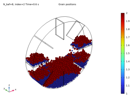
Locate the Animation Editing section. From the Parameter value (N_baf,index) list, choose 2: N_baf=8, index=2.
8
Click the  Play button in the Graphics toolbar. This plays the animation of the grain mixing with 8 baffles.
Application Builder
The mixing indices can be computed using an Application Method. These may be added to an existing model via a Model Method using the Application Builder. Note that the Application Builder is only available in the Windows® version of the COMSOL Desktop. But once the Model Method is created, it can be run in both the Linux and Mac versions.
In the Home toolbar, click  Application Builder.
Methods
The code for the computing and plotting the mixing indices can be simplified by using utility classes.
util1
1
In the Home toolbar, click  More Libraries and choose Utility Class.
2
In the Application Builder window, right-click util1 and choose Edit.
3
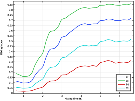
Copy the code for the utilities createGrid, createGrainEval, updateDatsets, getPlotFeature, plotMixingIndex and createGridDataSets and paste it into the Utility Class editor for util1.
/** Create the bins for the samples **/
 public static double[][] createGrid(int[] nbins, double[][] limits) {
   double[][] bins = new double[3][];
   for (int i = 0; i < 3; i++)
   {
     bins[i] = new double[nbins[i]];
     double range = limits[i][1]-limits[i][0];
     double margin = 1e-10*range;
     bins[i][0] = limits[i][0]-margin;
     for (int j = 0; j < nbins[i]; j++) {
       bins[i][j] = limits[i][0]+j*range/(nbins[i]-1);
     }
     bins[i][nbins[i]-1] = limits[i][1]+margin;
   }
   return bins;
 }
 
 /** Create the Grain evaluations */
 public static NumericalFeature createGrainEval(String tag, NumericalFeatureList numericalList, int idx) {
   NumericalFeature grn;
   if (numericalList.index(tag) != -1)
     numericalList.remove(tag);
   
   grn = model.result().numerical().create(tag, "Grain");
   grn.setIndex("looplevelinput", "all", 0);
   grn.set("data", "gran2");
   grn.setIndex("looplevelinput", "manualindices", 1);
   grn.setIndex("looplevelindices", idx, 1);
   return grn;
 }
 
 /** Create or update the grid datasets. */
 public static void updateDatsets(int i, String[] param,
                                  String[] tagList, String idx) {
   DatasetFeature dataFeature;
   if (model.result().dataset().index(tagList[i]+idx) == -1) {
     dataFeature = model.result().dataset().create(tagList[i]+idx, "Grid1D");
     dataFeature.label(tagList[i]+idx);
   }
   else {
     dataFeature = model.result().dataset().get(tagList[i]+idx);
   }
   with(dataFeature);
     set("source", "function");
     set("function", tagList[i]+idx);
     set("parmin1", param[0]);
     set("parmax1", param[1]);
     set("par1", param[2]);
   endwith();
 }
 
 /** Create or get the plot feature. */
 public static ResultFeature getPlotFeature(String pLabel) {
   ResultFeature miPlot;
   String pTag = "";
   String pLabel_in = pLabel;
   String[] rTag = model.result().tags();
   
   for (int i = 0; i < rTag.length; i++) {
     if (findIn(model.result(rTag[i]).label(), pLabel_in) > -1) {
       pTag = rTag[i];
       pLabel = model.result(rTag[i]).label();
     }
   }
   
   if (pTag.length() == 0) {
     pTag = model.result().uniquetag("pg");
     miPlot = model.result().create(pTag, "PlotGroup1D");
     miPlot.label(pLabel);
     with(miPlot);
       set("data", "none");
       set("titletype", "none");
       set("legendpos", "upperright");
       set("ylabelactive", true);
       set("ylabel", "Mixing index");
     endwith();
   }
   else
     miPlot = model.result().get(pTag);
   return miPlot;
 }
 
 /* Add the line plots to the Mixing Index plot group */
 public static void plotMixingIndex(String[] miList, String[] miTags, String idx)
 {
   // Create or get the MI plot group
   ResultFeature miPlot = util1.getPlotFeature("Mixing Index,"+idx);
   // Create or get the line graphs
   ResultFeatureList miPlotList = miPlot.feature();
   
   int num_plots = miList.length;
   for (int i = 0; i < num_plots; i++) {
     if (miPlotList.index(miTags[i]) == -1) {
       ResultFeature miPlotLine = miPlot.create(miTags[i], "LineGraph");
       miPlotLine.label(miList[i]);
       String expr_str = miTags[i]+idx+"(out)";
       with(miPlotLine);
         set("xdata", "expr");
         set("expr", expr_str);
         set("xdataexpr", "out");
         set("xdatadescractive", true);
         set("xdatadescr", "Mixing time (s)");
         set("data", miTags[i]+idx);
         set("legend", true);
         set("autodescr", true);
         set("autosolution", false);
         set("descractive", true);
         set("descr", miTags[i]);
         set("smooth", "none");
         set("resolution", "norefine");
         set("linewidth", 2);
       endwith();
     }
   }
 }
 
 /* Create the interpolation functions and the grid data sets*/
 public static void createGridDataSets(String[] miTags, int num_steps, double[][] MI, String idx) {
   FunctionFeatureList functionList = model.func();
   FunctionFeature functionFeature;
   
   NodeGroupList grpList = model.nodeGroup();
   NodeGroup grp;
   String grpTag = "grp"+idx+"baf";
   if (grpList.index(grpTag) == -1) {
     grp = model.nodeGroup().create(grpTag, "GlobalDefinitions");
     model.nodeGroup(grpTag).set("type", "func");
   }
   else
     grp = grpList.get(grpTag);
   
   for (int i = 0; i < 4; i++) {
     if (functionList.index(miTags[i]+idx) == -1) {
       functionFeature = functionList.create(miTags[i]+idx, "Interpolation");
       functionFeature.label(miTags[i]+idx);
       with(functionFeature);
         set("funcname", miTags[i]+idx);
         set("interp", "piecewisecubic");
         set("extrap", "const");
         set("defineprimfun", true);
       endwith();
     }
     else {
       functionFeature = functionList.get(miTags[i]+idx);
     }
     
     with(functionFeature);
       set("table", new String[0][0]);
       for (int k = 0; k < num_steps; k++) {
         setIndex("table", MI[k][0], k, 0);
         setIndex("table", MI[k][i+1], k, 1);
       }
     endwith();
     
     String pmin = toString(MI[0][0]);
     String pmax = toString(MI[num_steps-1][0]);
     String[] params = {pmin, pmax, "out"};
     util1.updateDatsets(i, params, miTags, idx);
     
     grp.add("func", miTags[i]+idx);
     grp.label(idx+" baffles");
   }
 }
Global Method
Now add a Model Method to compute the mixing indices that uses the utility functions.
1
In the Home toolbar, click New Method and choose Global Method.
2
In the Global Method dialog, type computeMI in the Name text field.
3
4
5
In the Settings window for Method, locate the Inputs and Output section.
6
Find the Inputs subsection. Click  Add.
7
8
9
10
11
12
13
14
15
computeMI
1
In the Application Builder window, under Methods click computeMI.
2
Copy the code for method computeMI and paste it into the Method editor.
int bafIdx = Integer.parseInt(baf_idx);
 String[] plistarr = model.study("std2").feature("param").getStringArray("plistarr")[0].split(" ");
 if (bafIdx > plistarr.length)
   error("Invalid baf_idx");
 String numBaf = plistarr[bafIdx-1];
 
 double xmin = -1*model.param().evaluate("R_d");
 double xmax = 1*model.param().evaluate("R_d");
 double ymin = 0;
 double ymax = model.param().evaluate("W_d");
 double zmin = -1*model.param().evaluate("R_d");
 double zmax = 1*model.param().evaluate("R_d");
 
 double[][] limits = new double[][]{{xmin, xmax}, {ymin, ymax}, {zmin, zmax}};
 
 // Calculate the overall grain fraction (p)
 NumericalFeatureList numericalList = model.result().numerical();
 NumericalFeature gev;
 if (numericalList.index("gev1") == -1)
   gev = model.result().numerical().create("gev1", "EvalGlobal");
 else
   gev = numericalList.get("gev1");
 
 gev.set("data", "gran2");
 gev.setIndex("expr", "gran.sum(1)", 0); // Total number of grains
 gev.setIndex("expr", "gran.rel1.Ntf", 1); // Number of small grains
 gev.setIndex("looplevelinput", "first", 0);
 double[][] num_grains = gev.getReal();
 double num_tot = num_grains[0][0];
 double num_i = num_grains[1][0];
 
 double p = num_i/num_tot;
 
 // Create the grid for the sampling.
 int nx = Integer.parseInt(ncells_x);
 int ny = Integer.parseInt(ncells_y);
 int nz = Integer.parseInt(ncells_z);
 double output_ts = Double.parseDouble(output_timestep);
 
 int[] nbins = {nx, ny, nz};
 double[][] bins = util1.createGrid(nbins, limits);
 double[][][] ni = new double[nx][ny][nz]; // Number of target type grains
 double[][][] Ni = new double[nx][ny][nz]; // Overall number of grains
 
 // Get the grain positions and sidx
 NumericalFeature grn1 = util1.createGrainEval("grn1", numericalList, bafIdx);
 NumericalFeature grn2 = util1.createGrainEval("grn2", numericalList, bafIdx);
 NumericalFeature grn3 = util1.createGrainEval("grn3", numericalList, bafIdx);
 NumericalFeature grn4 = util1.createGrainEval("grn4", numericalList, bafIdx);
 
 grn1.set("expr", "qx");
 grn2.set("expr", "qy");
 grn3.set("expr", "qz");
 grn4.set("expr", "gran.sidx");
 
 double[][] qx = grn1.computeResult()[0];
 double[][] qy = grn2.computeResult()[0];
 double[][] qz = grn3.computeResult()[0];
 double[][] sidx = grn4.computeResult()[0];
 
 int num_steps = qx.length;
 double[][] MI = new double[num_steps][5];
 
 double[] bin_size = new double[3];
 for (int i = 0; i < 3; i++) {
   if (nbins[i] > 1)
     bin_size[i] = bins[i][1]-bins[i][0];
   else
     bin_size[i] = limits[i][1]-limits[i][0];
 }
 
 for (int iT = 0; iT < num_steps; iT++) { // Timestep loop
   // Initialize the sample counts
   for (int i = 0; i < nbins[0]; i++) {
     for (int j = 0; j < nbins[1]; j++) {
       for (int k = 0; k < nbins[2]; k++) {
         ni[i][j][k] = 0;
         Ni[i][j][k] = 0;
       }
     }
   }
   
   // Sort the grains into the samples
   for (int i = 0; i < qx[0].length; i++) {
     int ix = -1; int iy = -1; int iz = -1;
     ix = (int) ((qx[iT][i]-limits[0][0])/bin_size[0]);
     iy = (int) ((qy[iT][i]-limits[1][0])/bin_size[1]);
     iz = (int) ((qz[iT][i]-limits[2][0])/bin_size[2]);
     
     if (sidx[0][i] == 1.0)
       ni[ix][iy][iz] += 1;
     Ni[ix][iy][iz] += 1;
   }
   
   int check = 0, num_samples = 0;
   double temp, sigma2 = 0;
   for (int i = 0; i < nx; i++) {
     for (int j = 0; j < ny; j++) {
       for (int k = 0; k < nz; k++) {
         check += Ni[i][j][k];
         if (Ni[i][j][k] > 0) {
           temp = Math.pow((ni[i][j][k]/Ni[i][j][k]-p), 2);
           sigma2 += (Ni[i][j][k]/num_tot)*temp;
           num_samples += 1;
         }
       }
     }
   }
   assert(check == num_tot);
   
   // Sample statistics
   double avg_size = num_tot/num_samples;
   double sigma = Math.sqrt(sigma2);
   double sigma_0 = Math.sqrt(p*(1-p));
   double sigma_r = Math.sqrt(p*(1-p)/avg_size);
   
   double t_fill = model.param().evaluate("t_fill");
   
   // Mixing indices
   MI[iT][0] = t_fill+iT*output_ts; // Mixing time
   MI[iT][1] = (sigma_0-sigma)/(sigma_0-sigma_r); // Kramer Index
   MI[iT][2] = (Math.pow(sigma_0, 2)-sigma2)/(Math.pow(sigma_0, 2)-Math.pow(sigma_r, 2)); // Lacey Index
   MI[iT][3] = ((sigma_0/sigma)-1)/((sigma_0/sigma_r)-1); // Beaudry Index
   MI[iT][4] = (Math.log(sigma_0)-Math.log(sigma))/(Math.log(sigma_0)-Math.log(sigma_r)); // Valentin Index
 }
 
 String[] miList = new String[]{"KramerIndex", "LaceyIndex", "BeaudryIndex", "ValentinIndex"};
 String[] miTags = new String[]{"Kr", "Lc", "Bd", "Vl"};
 
 util1.createGridDataSets(miTags, num_steps, MI, numBaf);
 util1.plotMixingIndex(miList, miTags, numBaf);
Methods
1
In the Home toolbar, click  Model Builder to switch to the main desktop.
Add a Method Call to computeMI in order to run it.
2
In the Developer toolbar, click  Method Call and choose computeMI.
Global Definitions
Compute Mixing Indices
1
In the Model Builder window, under Global Definitions click ComputeMI 1.
2
In the Settings window for Method Call, type Compute Mixing Indices in the Label text field.
The computeMI method accepts five arguments. The first argument is the index in the parameter sweep (number of baffles). The method computes and plots the four mixing indices as a function of time for the model with the corresponding number of baffles. The next three arguments are used to discretize the model geometry into various samples. The final argument is the time step in the Output times. Run the model method for the two parameter indices in the sweep.
3
Click  Run. Click Yes if the Confirm Run Method dialogue box appears. This produces four Interpolation features that are grouped under the name 4 baffles which are then used to create the plots of the mixing indices as a function of time.
Results
Mixing Index,4
1
In the Model Builder window, under Results click Mixing Index,4.
2
In the Settings window for 1D Plot Group, locate the Legend section.
3
From the Position list, choose Lower right.
4
In the Mixing Index,4 toolbar, click  Plot. Click Yes if the Confirm Run Method dialogue box appears. The plot of the mixing indices as a function of time with four baffles should look like Figure 4.
Global Definitions
Compute Mixing Indices
1
In the Model Builder window, under Global Definitions click Compute Mixing Indices.
2
In the Settings window for Method Call, locate the Inputs section.
3
In the Index of sweep text field, type 2.
4
Click  Run. This produces four Interpolation features that are grouped under the name 8 baffles which are then used to create the plots of the mixing indices as a function of time.
Results
Mixing Index,8
1
In the Model Builder window, under Results click Mixing Index,8.
2
In the Settings window for 1D Plot Group, locate the Legend section.
3
From the Position list, choose Lower right.
4
In the Mixing Index,8 toolbar, click  Plot. The plot of the mixing indices as a function of time with eight baffles should look like Figure 5.
Effect of Baffles
1
In the Results toolbar, click  1D Plot Group.
2
In the Settings window for 1D Plot Group, type Effect of Baffles in the Label text field.
3
Locate the Data section. From the Dataset list, choose None.
4
Locate the Plot Settings section.
5
Select the y-axis label checkbox. In the associated text field, type Kramer Index.
6
Locate the Legend section. From the Position list, choose Lower right.
4 Baffles
1
In the Effect of Baffles toolbar, click  Line Graph.
2
In the Settings window for Line Graph, type 4 Baffles in the Label text field.
3
Locate the Data section. From the Dataset list, choose Kr4.
4
Locate the y-Axis Data section. In the Expression text field, type Kr4(out).
5
Select the Description checkbox. In the associated text field, type 4 baffles.
6
Locate the x-Axis Data section. From the Parameter list, choose Expression.
7
In the Expression text field, type out.
8
Select the Description checkbox. In the associated text field, type Mixing time (s).
9
Click to expand the Legends section. Select the Show legends checkbox.
10
Find the Include subsection. Clear the Solution checkbox.
11
Select the Description checkbox.
8 Baffles
1
Right-click 4 Baffles and choose Duplicate.
2
In the Settings window for Line Graph, type 8 Baffles in the Label text field.
3
Locate the Data section. From the Dataset list, choose Kr8.
4
Locate the y-Axis Data section. In the Expression text field, type Kr8(out).
5
In the Description text field, type 8 baffles.
6
In the Effect of Baffles toolbar, click  Plot. The plot should look like Figure 6.