PDF

Mixing Grains in a Ribbon Mixer
Introduction
A ribbon mixer (sometimes referred to as a ribbon blender) is a mechanical device that is commonly used to mix different types of granular material. Ribbon mixers are widely used across various industries including food processing, pharmaceuticals, chemical industries, agriculture, cosmetics, and plastics.
A ribbon mixer typically consists of a U-shaped trough with a rotating central shaft along its length. The central shaft has helical ribbons (blades) attached to it that helps in mixing the material. Mixing in a ribbon mixer is complex phenomenon and is affected by several factors including the material and contact properties of the grains and the walls, filling level of the trough, and rotational speed. The design of the ribbons can also have a significant impact on the types of mixing behavior, and their efficiencies. One common class of ribbon mixers involve the use of two ribbons of different diameters, commonly referred to as a double ribbon mixer. The inner and outer helical ribbons often have opposing handedness. This promotes axial mixing as the ribbons push the grains along different axial directions.
This example uses the Granular Flow interface to model the filling of a U-shaped trough with two types of grains, followed by their mixing induced by the rotational motion of the ribbons. This model also shows the use of a Bounding Box feature to avoid scenarios that may adversely affect the performance of the Granular Flow interface. The extent of the overall mixing is quantified by the evaluation of the Kramer mixing index (Ref. 1). An additional indicator of the extent of axial mixing is also demonstrated.
Model Definition
The geometry consists of an U-shaped trough with a casing radius of 12 cm and a length of 33.2 cm. A central shaft of radius 0.8 cm runs through the length of the trough. Two helical ribbons are attached to the shaft along with support rods to hold the ribbons in place. The outer helix has a major radius of 10.25 cm is left handed, while the inner helix is left handed and has a major radius of 6.25 cm. The two blades have a pitch of 15 cm and 7.5 cm respectively. The top of the trough has four rectangular slits for releasing grains into the trough. These inlets can be closed during the mixing of the grains. The geometry is presented in Figure 1.
Two types of grains, one having a radius of 10 mm and another of 9 mm are considered. The trough is first filled with 4000 larger grains in a uniform manner. This is followed by the release of the smaller grains through each of the four inlets. A total of 100 such grains (per inlet) are released every 0.08 s up to 1.0 s. The grains are characterized by their release feature, thus leading to a mixture of five types of grains. All the grains are allowed to settle for a total of 2.0 s. The ribbon mixer is then rotated at an angular speed of 60 rpm for a total of 50 s to allow the grains to mix.
Figure 1: Model geometry.
The extent of the mixing is quantified by a mixing index, which is a parameter ranging from 0 indicating a completely segregated mixture, to a value of 1 indicating a fully mixed state. The evaluation procedure outlined in Ref. 1 is followed in this model. The process usually begins with evaluating the composition of a number of samples from the mixture. The domain is divided into a number of grid cells and the set of grains contained in each cell is treated as a sample.
For each sample, p is defined as the number fraction of the target grain type. The mixing index is then evaluated as a statistical expression of the variance in the composition across the samples. Furthermore, σ is defined as the standard deviation of the concentration across all the samples. For a completely segregated mixture, the standard deviation is . Similarly, the standard deviation in a fully mixed state is given by where n is the average size of the sample.
The Kramer mixing index can then be defined as
Notes on the COMSOL Implementation
The model is solved using two studies. In the first study, the grains are released into the trough using one Release feature and four Inlet features to release the grains sequentially. Each grain has a release index variable (gran.grf) associated with it which indicates the release feature that introduced that grain. This variable is used to divide the grains mixture into five types of grains. These grains are allowed to settle under the Gravity force. During this process, some grains may bounce off of the blades and exit the trough through the Inlet boundaries. These grains can continue moving away from the trough, which can adversely affect the performance of the Granular Flow interface. A Bounding Box feature is used to remove such grains from the simulation.
The degrees of freedom of the grains at the end of this study are used to initialize the second study in which the ribbon blade is allowed to rotate. The blade rotation is controlled by the Wall Movement settings in the Wall feature. An additional Wall feature is used to cover the inlet boundaries during this study to ensure that no grains leave the domain during the mixing process. Note that this feature needs to be disabled in the first study to allow the grains to be released along the inlet boundaries. Finally, since this feature prevents grains from exiting the trough, the Bounding Box feature can be disabled in this study.
Once the second study is completed, the evaluation of the Kramer mixing index requires statistical analysis on the various samples in the mixture. This is achieved by adding and running a Model Method.
Note: Model methods can only be set up in the COMSOL Desktop environment on the Windows version of COMSOL Multiphysics.
The maximum allowed time step taken by the Time-Dependent Solver in Granular Flow is often limited by the collision time scales of the grain-grain and grain-wall interactions. The collision time scales are often strongly dependent on the material properties such as density and Young’s modulus with stiffer grains generally exhibiting smaller collision times, thus requiring even smaller time steps. In many instances however, the stiffness of the grains and walls have a very limited effect on the bulk behavior of granular materials, and the materials can thus be made artificially less stiff in order to speed up the simulations.
Results and Discussion
Figure 2 shows the trough with the stationary ribbon blade and filled with the five types of grains. The grains are colored based on their release index. The dark blue grains were released directly into the domain using the Release feature, while the rest of the grains were released along the top surface though four Inlet features. For the most part, the five types of grains are completely separated.
Figure 2: Trough filled with the grains. The grains are colored by their release index.
Once the ribbon rotation is enabled, the wall forces push the grains both radially and axially. These wall forces, combined with the gravitational forces facilitate the mixing of the grains. The corresponding mixture at the end of 50.0 s of blade rotation is presented in Figure 3, where mixing can be observed. Note that the mixing is only partial and patches of homogeneity can still be observed in this mixture.
Figure 3: Grain positions after rotational mixing of 50 s.
The design of the helical blades ensures that the grains are pushed along the axis in both the directions. This can be visualized by evaluating the average axial position of the grains of each type. The normalized values as a function of time for the grains released through the inlets are plotted in Figure 4. It can be seen that initially, the average axial positions for each grain type are close to 0.25 or 0.75. This is because the axial distributions of each grain type is uniform and extends only up to half the axial length. As mixing occurs, all four curves converge towards a value approaching 0.5 indicating that the axial distribution of the grains have smoothened out and extend from one end to the other. It is clear from this plot the axial mixing is not yet complete.
Finally, Figure 5 presents the plot of the Kramer index as a function of time for each of the five grain types. As expected, the index is close to 0 before the mixing starts, and rises steadily until it saturates at a value close to 1.0 as mixing occurs.
Figure 4: Normalized average axial positions of four grain types.
Figure 5: Evolution of the Kramer mixing index for each type of grain.
Reference
1. X. Jin, G.R. Chandratilleke, S.Wang, and Y. Shen, “DEM investigation of mixing indices in a ribbon mixer,” Particuology, vol. 60, pp. 37–47, 2022.
Application Library path: Granular_Flow_Module/Mixing_and_Separation/ribbon_mixer
Modeling Instructions
From the Main Toolbar menu, choose New.
New
In the New window, click  Model Wizard.
Model Wizard
1
In the Model Wizard window, click  3D.
2
In the Select Physics tree, select Fluid Flow > Granular Flow (gran).
3
Click Add.
4
Click  Study.
5
In the Select Study tree, select General Studies > Time Dependent.
6
Geometry 1
Insert the prepared geometry sequence from file. You can read the instructions for creating the geometry in the appendix.
1
In the Geometry toolbar, click Insert Sequence and choose Insert Sequence.
2
3
In the Geometry toolbar, click  Build All.
Global Definitions
Geometry Parameters
1
In the Model Builder window, under Global Definitions click Parameters 1.
2
In the Settings window for Parameters, type Geometry Parameters in the Label text field.
Model Parameters
1
In the Home toolbar, click  Parameters and choose Add > Parameters.
2
In the Settings window for Parameters, type Model Parameters in the Label text field.
3
Locate the Parameters section. Click  Load from File.
4
5
Click the  Transparency button in the Graphics toolbar.
6
Click the  Zoom Extents button in the Graphics toolbar. The geometry should look like Figure 1.
Materials
Grains
1
In the Materials toolbar, click  Blank Material.
2
In the Settings window for Material, type Grains in the Label text field.
3
Click to expand the Material Properties section. In the Material properties tree, select Basic Properties > Density.
4
Click  Add to Material.
5
In the Material properties tree, select Basic Properties > Poisson’s Ratio.
6
Click  Add to Material.
7
In the Material properties tree, select Basic Properties > Young’s Modulus.
8
Click  Add to Material.
9
Locate the Material Contents section. In the table, enter the following settings:
Walls
1
In the Materials toolbar, click  Blank Material.
2
In the Settings window for Material, type Walls in the Label text field.
3
Locate the Geometric Entity Selection section. From the Geometric entity level list, choose Boundary.
4
From the Selection list, choose All boundaries.
5
Locate the Material Contents section. In the table, enter the following settings:
Granular Flow (gran)
Grain Properties 1
1
In the Model Builder window, under Component 1 (comp1) > Granular Flow (gran) click Grain Properties 1.
2
In the Settings window for Grain Properties, locate the Granular Material Properties section.
3
From the Granular material list, choose Grains (mat1).
4
Locate the Size section. In the dg text field, type dg.
Grain Properties 2
1
In the Physics toolbar, click  Global and choose Grain Properties.
2
In the Settings window for Grain Properties, locate the Granular Material Properties section.
3
From the Granular material list, choose Grains (mat1).
4
Locate the Size section. In the dg text field, type dg*0.9.
Contact Between Grains 1
1
In the Model Builder window, click Contact Between Grains 1.
2
In the Settings window for Contact Between Grains, locate the Contact Properties section.
3
In the en text field, type en.
4
In the et text field, type et.
5
In the μs text field, type mus.
6
In the μr text field, type mur.
7
In the μtw text field, type mutw.
Contact with Walls 1
1
In the Model Builder window, click Contact with Walls 1.
2
In the Settings window for Contact with Walls, locate the Contact Properties section.
3
In the en text field, type en.
4
In the et text field, type et.
5
In the μs text field, type mus.
6
In the μr text field, type mur.
7
In the μtw text field, type mutw.
Release 1
1
In the Physics toolbar, click  Domains and choose Release.
2
3
In the Settings window for Release, locate the Released Grain Properties section.
4
Inlet 1
1
In the Physics toolbar, click  Boundaries and choose Inlet.
2
3
In the Settings window for Inlet, locate the Release Times section.
4
In the Release times text field, type range(0,0.08,1.0).
5
Locate the Initial Values section. Specify the v0 vector as
6
Locate the Released Grain Properties section. In the table, enter the following settings:
7
Locate the Advanced Settings section. In the Number of release attempts per grain text field, type 25.
Inlet 2
1
Right-click Inlet 1 and choose Duplicate.
2
Inlet 3
1
Right-click Inlet 2 and choose Duplicate.
2
Inlet 4
1
Right-click Inlet 3 and choose Duplicate.
2
Outlet 1
1
In the Physics toolbar, click  Boundaries and choose Outlet.
2
Mixer Blades
1
In the Physics toolbar, click  Boundaries and choose Wall.
2
In the Settings window for Wall, type Mixer Blades in the Label text field.
3
Locate the Boundary Selection section. From the Selection list, choose Mixer Blades.
4
Locate the Wall Movement section. From the Wall motion list, choose Rotation.
5
In the ω text field, type om.
6
In the α0 text field, type -om*t_fill.
7
Specify the eax vector as
Inlet Gates
Next, add a Wall feature to effectively close the inlet boundaries once the trough is filled. This feature is disabled in the first study to allow the grains to enter the trough.
1
In the Physics toolbar, click  Boundaries and choose Wall.
2
In the Settings window for Wall, type Inlet Gates in the Label text field.
3
Bounding Box 1
1
In the Physics toolbar, click  Global and choose Bounding Box.
2
In the Settings window for Bounding Box, locate the Settings section.
3
In the x minimum text field, type -Rc*1.2.
4
In the x maximum text field, type Rc*1.2.
5
In the y minimum text field, type -2*offset.
6
In the y maximum text field, type L+2*offset.
7
In the z minimum text field, type -Rc-10*dg.
8
In the z maximum text field, type Rc*1.2+10*dg.
Study 1: Filling
1
In the Model Builder window, click Study 1.
2
In the Settings window for Study, type Study 1: Filling in the Label text field.
Step 1: Time Dependent
1
In the Model Builder window, under Study 1: Filling click Step 1: Time Dependent.
2
In the Settings window for Time Dependent, locate the Study Settings section.
3
In the Output times text field, type range(0,0.25,t_fill).
4
Locate the Physics and Variables Selection section. Select the Modify model configuration for study step checkbox.
5
In the tree, select Component 1 (comp1) > Granular Flow (gran) > Mixer Blades and Component 1 (comp1) > Granular Flow (gran) > Inlet Gates.
6
Click  Disable.
7
In the Study toolbar, click  Compute.
Results
Grain Positions (gran)
In the Model Builder window, expand the Grain Positions (gran) node.
Color Expression 1
1
In the Model Builder window, expand the Results > Grain Positions (gran) > Grain Positions 1 node, then click Color Expression 1.
2
In the Settings window for Color Expression, locate the Expression section.
3
In the Expression text field, type gran.grf.
4
In the Grain Positions (gran) toolbar, click  Plot.
5
Click the  Transparency button in the Graphics toolbar. The plot should look like Figure 2.
Add Study
1
In the Home toolbar, click  Add Study to open the Add Study window.
2
Go to the Add Study window.
3
Find the Studies subsection. In the Select Study tree, select General Studies > Time Dependent.
4
Click the Add Study button in the window toolbar.
5
In the Home toolbar, click  Add Study to close the Add Study window.
Study 2: Mixing
In the Settings window for Study, type Study 2: Mixing in the Label text field.
Step 1: Time Dependent
1
In the Model Builder window, under Study 2: Mixing click Step 1: Time Dependent.
2
In the Settings window for Time Dependent, locate the Study Settings section.
3
In the Output times text field, type range(t_fill,0.5,t_fill+t_mix).
4
Locate the Physics and Variables Selection section. Select the Modify model configuration for study step checkbox.
5
In the tree, select Component 1 (comp1) > Granular Flow (gran) > Bounding Box 1.
6
Click  Disable.
7
Click to expand the Values of Dependent Variables section. Find the Initial values of variables solved for subsection. From the Settings list, choose User controlled.
8
From the Method list, choose Solution.
9
From the Study list, choose Study 1: Filling, Time Dependent.
10
In the Study toolbar, click  Compute.
Results
Grain Positions (gran) 1
In the Model Builder window, expand the Results > Grain Positions (gran) 1 node.
Color Expression 1
1
In the Model Builder window, expand the Results > Grain Positions (gran) 1 > Grain Positions 1 node, then click Color Expression 1.
2
In the Settings window for Color Expression, locate the Expression section.
3
In the Expression text field, type gran.grf.
4
In the Grain Positions (gran) 1 toolbar, click  Plot. The plot should look like Figure 3.
Animation 1
1
In the Grain Positions (gran) 1 toolbar, click  Animation and choose Player.
2
In the Settings window for Animation, locate the Frames section.
3
From the Frame selection list, choose All.
4
Click the  Play button in the Graphics toolbar. This plays the animation of the grain mixing.
Average Positions
1
In the Results toolbar, click  1D Plot Group.
2
In the Settings window for 1D Plot Group, type Average Positions in the Label text field.
3
Locate the Data section. From the Dataset list, choose Grain 2.
4
Click to expand the Title section. From the Title type list, choose None.
5
Locate the Plot Settings section.
6
Select the x-axis label checkbox. In the associated text field, type Time (s).
7
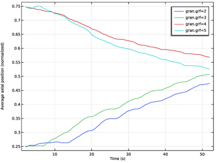
Select the y-axis label checkbox. In the associated text field, type Average axial position (normalized).
Grain 1
1
In the Average Positions toolbar, click  More Plots and choose Grain.
2
In the Settings window for Grain, locate the y-Axis Data section.
3
In the Expression text field, type (qy+offset)/L.
4
Select the Description checkbox. In the associated text field, type gran.grf=2.
5
Click to expand the Legends section. Select the Show legends checkbox.
6
Locate the Data Series Operation section. From the Operation list, choose Average.
Filter 1
1
In the Average Positions toolbar, click  Filter.
2
In the Settings window for Filter, locate the Grain Selection section.
3
From the Grains to include list, choose Logical expression.
4
In the Logical expression for inclusion text field, type gran.grf==2.
Grain 2
1
In the Model Builder window, under Results > Average Positions right-click Grain 1 and choose Duplicate.
2
In the Settings window for Grain, locate the y-Axis Data section.
3
In the Description text field, type gran.grf=3.
Filter 1
1
In the Model Builder window, expand the Grain 2 node, then click Filter 1.
2
In the Settings window for Filter, locate the Grain Selection section.
3
In the Logical expression for inclusion text field, type gran.grf==3.
Grain 3
1
In the Model Builder window, under Results > Average Positions right-click Grain 2 and choose Duplicate.
2
In the Settings window for Grain, locate the y-Axis Data section.
3
In the Description text field, type gran.grf=4.
Filter 1
1
In the Model Builder window, expand the Grain 3 node, then click Filter 1.
2
In the Settings window for Filter, locate the Grain Selection section.
3
In the Logical expression for inclusion text field, type gran.grf==4.
Grain 4
1
In the Model Builder window, under Results > Average Positions right-click Grain 3 and choose Duplicate.
2
In the Settings window for Grain, locate the y-Axis Data section.
3
In the Description text field, type gran.grf=5.
Filter 1
1
In the Model Builder window, expand the Grain 4 node, then click Filter 1.
2
In the Settings window for Filter, locate the Grain Selection section.
3
In the Logical expression for inclusion text field, type gran.grf==5.
4
In the Average Positions toolbar, click  Plot. The plot should look like Figure 4.
Application Builder
The mixing indices can be computed using an Application Method. These may be added to an existing model via a Model Method using the Application Builder. Note that the Application Builder is only available in the Windows® version of the COMSOL Desktop. But once the Model Method is created, it can be run in both the Linux and Mac versions.
In the Home toolbar, click  Application Builder.
Methods
The code for the computing and plotting the mixing indices can be simplified by using utility classes.
util1
1
In the Home toolbar, click  More Libraries and choose Utility Class.
2
In the Application Builder window, right-click util1 and choose Edit.
3
Copy the code for the utilities createGrid, createGrainEval, updateDatsets, getPlotFeature, plotMixingIndex and createGridDataSets and paste it into the Utility Class editor for util1.
/** Create the bins for the samples **/
 public static double[][] createGrid(int[] nbins, double[][] limits) {
   double[][] bins = new double[3][];
   for (int i = 0; i < 3; i++)
   {
     bins[i] = new double[nbins[i]];
     double range = limits[i][1]-limits[i][0];
     double margin = 1e-10*range;
     bins[i][0] = limits[i][0]-margin;
     for (int j = 0; j < nbins[i]; j++) {
       bins[i][j] = limits[i][0]+j*range/(nbins[i]-1);
     }
     bins[i][nbins[i]-1] = limits[i][1]+margin;
   }
   return bins;
 }
 
 /** Create the Grain evaluations */
 public static NumericalFeature createGrainEval(String tag, NumericalFeatureList numericalList) {
   NumericalFeature grn;
   if (numericalList.index(tag) != -1)
     numericalList.remove(tag);
   
   grn = model.result().numerical().create(tag, "Grain");
   grn.setIndex("looplevelinput", "all", 0);
   grn.set("data", "gran2");
   return grn;
 }
 
 /** Create or update the grid datasets. */
 public static void updateDatsets(int i, String[] param,
                                  String[] tagList, String idx) {
   DatasetFeature dataFeature;
   if (model.result().dataset().index(tagList[i]+idx) == -1) {
     dataFeature = model.result().dataset().create(tagList[i]+idx, "Grid1D");
     dataFeature.label(tagList[i]+idx);
   }
   else {
     dataFeature = model.result().dataset().get(tagList[i]+idx);
   }
   with(dataFeature);
     set("source", "function");
     set("function", tagList[i]+idx);
     set("parmin1", param[0]);
     set("parmax1", param[1]);
     set("par1", param[2]);
   endwith();
 }
 
 /** Create or get the plot feature. */
 public static ResultFeature getPlotFeature(String pLabel) {
   ResultFeature miPlot;
   String pTag = "";
   String pLabel_in = pLabel;
   String[] rTag = model.result().tags();
   
   for (int i = 0; i < rTag.length; i++) {
     if (findIn(model.result(rTag[i]).label(), pLabel_in) > -1) {
       pTag = rTag[i];
       pLabel = model.result(rTag[i]).label();
     }
   }
   
   if (pTag.length() == 0) {
     pTag = model.result().uniquetag("pg");
     miPlot = model.result().create(pTag, "PlotGroup1D");
     miPlot.label(pLabel);
     with(miPlot);
       set("data", "none");
       set("titletype", "none");
       set("legendpos", "upperright");
       set("ylabelactive", true);
       set("ylabel", "Mixing index");
     endwith();
   }
   else
     miPlot = model.result().get(pTag);
   return miPlot;
 }
 
 /* Add the line plots to the Mixing Index plot group */
 public static void plotMixingIndex(String[] miList, String[] miTags, String idx)
 {
   // Create or get the MI plot group
   ResultFeature miPlot = util1.getPlotFeature("Mixing Index");
   // Create or get the line graphs
   ResultFeatureList miPlotList = miPlot.feature();
   
   int num_plots = miList.length;
   for (int i = 0; i < num_plots; i++) {
     if (miPlotList.index(miTags[i]+idx) == -1) {
       ResultFeature miPlotLine = miPlot.create(miTags[i]+idx, "LineGraph");
       miPlotLine.label("gran.grf="+idx);
       String expr_str = miTags[i]+idx+"(out)";
       with(miPlotLine);
         set("xdata", "expr");
         set("expr", expr_str);
         set("xdataexpr", "out");
         set("xdatadescractive", true);
         set("xdatadescr", "Time (s)");
         set("data", miTags[i]+idx);
         set("descr", "gran.grf="+idx);
         set("legend", true);
         set("autodescr", true);
         set("autosolution", false);
         set("descractive", true);
         set("smooth", "none");
         set("resolution", "norefine");
         set("linewidth", 2);
       endwith();
     }
   }
 }
 
 /* Create the interpolation functions and the grid data sets*/
 public static void createGridDataSets(String[] miTags, int num_steps, double[][] MI, String idx) {
   FunctionFeatureList functionList = model.func();
   FunctionFeature functionFeature;
   
   for (int i = 0; i < miTags.length; i++) {
     if (functionList.index(miTags[i]+idx) == -1) {
       functionFeature = functionList.create(miTags[i]+idx, "Interpolation");
       functionFeature.label(miTags[i]+idx);
       with(functionFeature);
         set("funcname", miTags[i]+idx);
         set("interp", "piecewisecubic");
         set("extrap", "const");
         set("defineprimfun", true);
       endwith();
     }
     else {
       functionFeature = functionList.get(miTags[i]+idx);
     }
     
     with(functionFeature);
       set("table", new String[0][0]);
       for (int k = 0; k < num_steps; k++) {
         setIndex("table", MI[k][0], k, 0);
         setIndex("table", MI[k][i+1], k, 1);
       }
     endwith();
     
     String pmin = toString(MI[0][0]);
     String pmax = toString(MI[num_steps-1][0]);
     String[] params = {pmin, pmax, "out"};
     util1.updateDatsets(i, params, miTags, idx);
   }
 }
Global Method
Now add a Model Method to compute the mixing indices that uses the utility functions.
1
In the Home toolbar, click New Method and choose Global Method.
2
In the Global Method dialog, type computeMI in the Name text field.
3
4
5
In the Settings window for Method, locate the Inputs and Output section.
6
Find the Inputs subsection. Click  Add.
7
8
9
10
11
12
13
computeMI
1
In the Application Builder window, under Methods click computeMI.
2
Copy the code for method computeMI and paste it into the Method editor.
int tprf = Integer.parseInt(target);
 // Calculate the overall grain fraction (p)
 NumericalFeatureList numericalList = model.result().numerical();
 NumericalFeature gev;
 if (numericalList.index("gev1") == -1)
   gev = model.result().numerical().create("gev1", "EvalGlobal");
 else
   gev = numericalList.get("gev1");
 
 gev.set("data", "gran2");
 gev.setIndex("expr", "gran.sum(1)", 0); // All grains
 gev.setIndex("expr", "gran.sum(gran.grf=="+target+")", 1); // Target grains
 gev.setIndex("looplevelinput", "first", 0);
 double[][] num_grains = gev.getReal();
 double num_tot = num_grains[0][0];
 double num_target = num_grains[1][0];
 
 double p = num_target/num_tot;
 
 GeomSequence geom = model.component("comp1").geom("geom1");
 String[] size = geom.feature("blk1").getStringArray("size");
 double Lx = model.param().evaluate(size[0]);
 double Ly = model.param().evaluate(size[1]);
 
 double[] basePoint = {0, 0, 0};
 basePoint[0] = -Lx/2;
 basePoint[1] = model.param().evaluate("offset");
 basePoint[2] = -Lx/2;
 
 double xmin, xmax, ymin, ymax, zmin, zmax;
 xmin = -Lx/2;
 xmax = Lx/2;
 ymin = -1*model.param().evaluate("offset");
 ymax = Ly;
 zmin = -Lx/2;
 zmax = model.param().evaluate(size[2]);
 
 double[][] limits = new double[][]{{xmin, xmax}, {ymin, ymax}, {zmin, zmax}};
 
 // Create the grid for the sampling.
 int nx = Integer.parseInt(ncells_x);
 int ny = Integer.parseInt(ncells_y);
 int nz = Integer.parseInt(ncells_z);
 int[] nbins = {nx, ny, nz};
 double[][] bins = util1.createGrid(nbins, limits);
 double[][][] ni = new double[nx][ny][nz]; // Number of target type grains
 double[][][] Ni = new double[nx][ny][nz]; // Overall number of grains
 
 // Get the grain positions and sidx
 NumericalFeature grn1 = util1.createGrainEval("grn1", numericalList);
 NumericalFeature grn2 = util1.createGrainEval("grn2", numericalList);
 NumericalFeature grn3 = util1.createGrainEval("grn3", numericalList);
 NumericalFeature grn4 = util1.createGrainEval("grn4", numericalList);
 
 grn1.set("expr", "qx");
 grn2.set("expr", "qy");
 grn3.set("expr", "qz");
 grn4.set("expr", "gran.grf");
 
 double[][] qx = grn1.computeResult()[0];
 double[][] qy = grn2.computeResult()[0];
 double[][] qz = grn3.computeResult()[0];
 double[][] prf = grn4.computeResult()[0];
 int num_steps = qx.length;
 
 // Get the output time parameters
 String tlist = model.study("std2").feature("time").getString("tlist");
 String[] tlist_arr = tlist.split(",");
 double t_beg = model.param().evaluate(tlist_arr[0].split("\\(")[1]);
 double dt = model.param().evaluate(tlist_arr[1]);
 
 double[][] MI = new double[num_steps][2];
 
 double[] bin_size = new double[3];
 for (int i = 0; i < 3; i++) {
   if (nbins[i] > 1)
     bin_size[i] = bins[i][1]-bins[i][0];
   else
     bin_size[i] = limits[i][1]-limits[i][0];
 }
 
 for (int iT = 0; iT < num_steps; iT++) { // Timestep loop
   // Initialize the sample counts
   for (int i = 0; i < nbins[0]; i++) {
     for (int j = 0; j < nbins[1]; j++) {
       for (int k = 0; k < nbins[2]; k++) {
         ni[i][j][k] = 0;
         Ni[i][j][k] = 0;
       }
     }
   }
   
   // Sort the grains into the samples
   for (int i = 0; i < qx[0].length; i++) {
     int ix = -1; int iy = -1; int iz = -1;
     ix = (int) ((qx[iT][i]-limits[0][0])/bin_size[0]);
     iy = (int) ((qy[iT][i]-limits[1][0])/bin_size[1]);
     iz = (int) ((qz[iT][i]-limits[2][0])/bin_size[2]);
     
     if (prf[0][i] == tprf)
       ni[ix][iy][iz] += 1;
     Ni[ix][iy][iz] += 1;
   }
   
   int check = 0, num_samples = 0;
   double temp, sigma2 = 0;
   for (int i = 0; i < nx; i++) {
     for (int j = 0; j < ny; j++) {
       for (int k = 0; k < nz; k++) {
         check += Ni[i][j][k];
         if (Ni[i][j][k] > 0) {
           temp = Math.pow((ni[i][j][k]/Ni[i][j][k]-p), 2);
           sigma2 += (Ni[i][j][k]/num_tot)*temp;
           num_samples += 1;
         }
       }
     }
   }
   assert(check == num_tot);
   
   // Sample statistics
   double avg_size = num_tot/num_samples;
   double sigma = Math.sqrt(sigma2);
   double sigma_0 = Math.sqrt(p*(1-p));
   double sigma_r = Math.sqrt(p*(1-p)/avg_size);
   
   // Mixing indices
   MI[iT][0] = t_beg+iT*dt; // Mixing time
   MI[iT][1] = (sigma_0-sigma)/(sigma_0-sigma_r); // Kramer Index
 }
 
 String[] miList = new String[]{"KramerIndex"};
 String[] miTags = new String[]{"Kr"};
 
 util1.createGridDataSets(miTags, num_steps, MI, target);
 util1.plotMixingIndex(miList, miTags, target);
Methods
1
In the Home toolbar, click  Model Builder to switch to the main desktop.
Add a Method Call to computeMI in order to run it.
2
In the Developer toolbar, click  Method Call and choose computeMI.
Global Definitions
Compute Mixing Indices
1
In the Model Builder window, under Global Definitions click ComputeMI 1.
2
In the Settings window for Method Call, type Compute Mixing Indices in the Label text field.
The computeMI method accepts five arguments. The first argument is the release index of the grains. The method computes and plots the Kramer mixing index as a function of time for the grains identified by the corresponding release index. The next three arguments are used to discretize the model geometry into various samples. Run the model method to calculate the mixing index for the grains characterized by the release feature index given by the first argument.
3
Click  Run. Click Yes if the Confirm Run Method dialogue box appears. This produces an Interpolation feature which is then used to create the plot of the mixing index as a function of time. Now, run the model method for the remaining four grain release features.
4
Locate the Inputs section. In the Target species index text field, type 2.
5
Click  Run. Click Yes if the Confirm Run Method dialogue box appears.
6
In the Target species index text field, type 3.
7
Click  Run. Click Yes if the Confirm Run Method dialogue box appears.
8
In the Target species index text field, type 4.
9
Click  Run. Click Yes if the Confirm Run Method dialogue box appears.
10
In the Target species index text field, type 5.
11
Click  Run. Click Yes if the Confirm Run Method dialogue box appears.
Results
Mixing Index
1
In the Model Builder window, under Results click Mixing Index.
2
In the Settings window for 1D Plot Group, locate the Legend section.
3
From the Position list, choose Lower right.
4
In the Mixing Index toolbar, click  Plot. The plot of the mixing indices as a function of time should look like Figure 5.
Appendix: Geometry Instructions
From the Main Toolbar menu, choose New.
New
In the New window, click  Model Wizard.
Model Wizard
1
In the Model Wizard window, click  3D.
2
Global Definitions
Parameters 1
1
In the Model Builder window, under Global Definitions click Parameters 1.
2
In the Settings window for Parameters, locate the Parameters section.
3
Click  Load from File.
4
Geometry 1
Cylinder 1 (cyl1)
1
In the Geometry toolbar, click  Cylinder.
2
In the Settings window for Cylinder, locate the Size and Shape section.
3
In the Radius text field, type Ra.
4
In the Height text field, type L.
5
Locate the Position section. In the y text field, type -offset.
6
Locate the Axis section. From the Axis type list, choose y-axis.
Cylinder 2 (cyl2)
1
In the Geometry toolbar, click  Cylinder.
2
In the Settings window for Cylinder, locate the Size and Shape section.
3
In the Radius text field, type Rs.
4
In the Height text field, type Rbo+bh*0.55.
5
Locate the Axis section. From the Axis type list, choose Cartesian.
6
In the z text field, type -1.
Array 1 (arr1)
1
In the Geometry toolbar, click  Transforms and choose Array.
2
3
In the Settings window for Array, locate the Size section.
4
In the y size text field, type n.
5
Locate the Displacement section. In the y text field, type n*p.
Cylinder 3 (cyl3)
1
In the Geometry toolbar, click  Cylinder.
2
In the Settings window for Cylinder, locate the Size and Shape section.
3
In the Radius text field, type Rs.
4
In the Height text field, type Rbi-bh/4.
5
Locate the Position section. In the y text field, type p/4.
Array 2 (arr2)
1
In the Geometry toolbar, click  Transforms and choose Array.
2
3
In the Settings window for Array, locate the Size section.
4
In the y size text field, type 2*n.
5
Locate the Displacement section. In the y text field, type p/2.
Helix 1 (hel1)
1
In the Geometry toolbar, click  Helix.
2
In the Settings window for Helix, locate the Size and Shape section.
3
In the Number of turns text field, type n.
4
In the Major radius text field, type Rbo.
5
In the Minor radius text field, type 0.
6
In the Axial pitch text field, type p.
7
From the Chirality list, choose Left-handed.
8
Locate the Axis section. From the Axis type list, choose y-axis.
Work Plane 1 (wp1)
1
In the Geometry toolbar, click  Work Plane.
2
In the Settings window for Work Plane, locate the Plane Definition section.
3
From the Plane list, choose yz-plane.
Work Plane 1 (wp1) > Plane Geometry
In the Model Builder window, click Plane Geometry.
Work Plane 1 (wp1) > Rectangle 1 (r1)
1
In the Work Plane toolbar, click  Rectangle.
2
In the Settings window for Rectangle, locate the Size and Shape section.
3
In the Width text field, type bw.
4
In the Height text field, type bh.
5
Locate the Position section. From the Base list, choose Center.
6
In the yw text field, type -Rbo.
7
Locate the Rotation Angle section. In the Rotation text field, type -alpha.
8
Click  Build Selected.
Work Plane 1 (wp1) > Rectangle 2 (r2)
1
Right-click Component 1 (comp1) > Geometry 1 > Work Plane 1 (wp1) > Plane Geometry > Rectangle 1 (r1) and choose Duplicate.
2
In the Settings window for Rectangle, locate the Position section.
3
In the yw text field, type -Rbi.
4
Click  Build Selected.
Work Plane 1 (wp1)
Click the  Transparency button in the Graphics toolbar.
Sweep 1 (swe1)
1
In the Geometry toolbar, click  Sweep.
2
On the object wp1, select Boundary 1 only.
3
In the Settings window for Sweep, locate the Spine Curve section.
4
Click to select the  Activate Selection toggle button for Edges to follow.
5
On the object hel1, select Edge 1 only.
6
Locate the Motion of Cross Section section. From the Twisting list, choose Follow projection of vector to normal plane.
7
In the y text field, type 1.
8
In the z text field, type 0.
9
Click  Build Selected.
Helix 2 (hel2)
1
In the Geometry toolbar, click  Helix.
2
In the Settings window for Helix, locate the Size and Shape section.
3
In the Number of turns text field, type 2*n.
4
In the Major radius text field, type Rbi.
5
In the Minor radius text field, type 0.
6
In the Axial pitch text field, type p/2.
7
Locate the Axis section. From the Axis type list, choose y-axis.
Sweep 2 (swe2)
1
In the Geometry toolbar, click  Sweep.
2
On the object wp1, select Boundary 2 only.
3
In the Settings window for Sweep, locate the Spine Curve section.
4
Click to select the  Activate Selection toggle button for Edges to follow.
5
Locate the Motion of Cross Section section. From the Twisting list, choose Follow projection of vector to normal plane.
6
In the y text field, type 1.
7
In the z text field, type 0.
8
On the object hel2, select Edge 1 only.
9
Click  Build Selected.
10
Click the  Zoom Extents button in the Graphics toolbar.
Mixer Blades
1
In the Geometry toolbar, click  Booleans and Partitions and choose Union.
2
In the Settings window for Union, type Mixer Blades in the Label text field.
3
Locate the Union section. From the Input objects list, choose All objects.
4
Clear the Keep interior boundaries checkbox.
5
Locate the Selections of Resulting Entities section. Select the Resulting objects selection checkbox.
6
From the Show in physics list, choose Boundary selection.
7
Click  Build Selected.
Cylinder 4 (cyl4)
1
In the Geometry toolbar, click  Cylinder.
2
In the Settings window for Cylinder, locate the Size and Shape section.
3
In the Radius text field, type Rc.
4
In the Height text field, type L.
5
Locate the Position section. In the y text field, type -offset.
6
Locate the Axis section. From the Axis type list, choose y-axis.
Block 1 (blk1)
1
In the Geometry toolbar, click  Block.
2
In the Settings window for Block, locate the Size and Shape section.
3
In the Width text field, type 2*Rc.
4
In the Depth text field, type L.
5
In the Height text field, type 1.2*Rc.
6
Locate the Position section. In the x text field, type -Rc.
7
In the y text field, type -offset.
Union 2 (uni2)
1
In the Geometry toolbar, click  Booleans and Partitions and choose Union.
2
Select the objects blk1 and cyl4 only.
Difference 1 (dif1)
1
In the Geometry toolbar, click  Booleans and Partitions and choose Difference.
2
3
In the Settings window for Difference, locate the Difference section.
4
Click to select the  Activate Selection toggle button for Objects to subtract.
5
6
Clear the Keep interior boundaries checkbox.
Work Plane 2 (wp2)
1
In the Geometry toolbar, click  Work Plane.
2
In the Settings window for Work Plane, locate the Plane Definition section.
3
From the Plane type list, choose Face parallel.
4
On the object dif1, select Boundary 6 only.
Work Plane 2 (wp2) > Plane Geometry
In the Model Builder window, click Plane Geometry.
Work Plane 2 (wp2) > Rectangle 1 (r1)
1
In the Work Plane toolbar, click  Rectangle.
2
In the Settings window for Rectangle, locate the Size and Shape section.
3
In the Width text field, type Rc-2*gap.
4
In the Height text field, type p.
5
Locate the Position section. In the xw text field, type -(Rc-gap).
6
In the yw text field, type -L/2+offset/2.
Work Plane 2 (wp2) > Array 1 (arr1)
1
In the Work Plane toolbar, click  Transforms and choose Array.
2
3
In the Settings window for Array, locate the Size section.
4
In the xw size text field, type 2.
5
In the yw size text field, type 2.
6
Locate the Displacement section. In the xw text field, type Rc.
7
In the yw text field, type L/2.
Work Plane 3 (wp3)
In the Model Builder window, right-click Geometry 1 and choose Work Plane.
Form Union (fin)
1
In the Geometry toolbar, click  Build All.
2
In the Model Builder window, click Form Union (fin).
3
Click in the Graphics window and then press Ctrl+D to clear all objects.
Partition Domains 1 (pard1)
1
In the Geometry toolbar, click  Booleans and Partitions and choose Partition Domains.
2
On the object fin, select Domain 1 only.
3
In the Settings window for Partition Domains, click  Build Selected.
4
In the Geometry toolbar, click  Cleanup Wizard.
Cleanup Wizard
1
Go to the Cleanup Wizard window.
2
Click the Apply button in the window toolbar.
3
Click the Apply button in the window toolbar.
4
Click the Done button in the window toolbar.