PDF

Powder Spreading Using a Moving Roller
Introduction
Additive manufacturing techniques such as powder bed fusion (PBF) rely on obtaining thin uniform layers of powdered materials. The quality and the consistency of the obtained powder bed has a significant impact on the quality of the manufacturing process. The factors affecting the quality of the bed include its density, homogeneity, and thickness as well as the presence of any defects. This crucial step is most often achieved by first generating a heap of the powdered material in front of the bed. A moving roller is then used to spread the material onto the bed. The geometry and speed of the roller can affect the quality of the powder bed.
This example uses the Granular Flow interface to model the formation of the grain heap and then its subsequent spreading using a cylindrical roller. The roller has a combined rotational and translational motion. The resulting powder bed is then analyzed to determine its quality based on its packing fraction. Additional packing characteristics such as the distribution of the grain center heights and the coordination numbers are also evaluated.
This model also demonstrates the process of restarting the granular flow simulations whereby the information of the grains from one study step is used as the initial conditions for a subsequent study step.
Model Definition
The geometry consists of three rectangular compartments. The first one houses the roller until it is ready to move. The grains are released into the middle compartment. The third compartment represents the powder bed. The length and the width of the middle compartment is 40 mm. The length of the powder bed is set to 200 mm, and the height of all the compartments is 60 mm. The roller has a diameter of 15 mm and is initially situated in the first compartment such that it has a gap of 3 mm from both its walls in the x direction. The geometry is presented in Figure 1. The two boundaries that separate the middle compartment from the other two represent gates that can be added and removed to alter the geometry.
A total of 20,000 grains, each having a diameter of 1 mm, are first released randomly into the middle compartment. The grains initially settle under the influence of gravity for 0.25 s to form a compact bed since the two gates are closed. Periodic boundary conditions are applied along the y directions to isolate the wall effects in this direction. Once the grains are settled, the two gates are lifted to allow the grains to form a stable heap. The heap formation time is 0.4 s.
Figure 1: Model geometry.
Finally, the roller blade is allowed to move with a translational speed of 100 mm/s for a total linear traversal length of 163 mm. The roller also rotates with an angular speed of 6 rad/s around its axis. This action causes the powder spreading and the formation of a compact powder bed.
Notes on COMSOL Implementation
The model is solved using three studies. In the first study, the grains are released into the middle compartment and are allowed to settle. The degrees of freedom of the grains at the end of this study are used to initialize the second study in which the gates are removed instantaneously to allow for the heap formation. The removal of these gates is achieved by using the Outlet feature. Once the heap is stable, the degrees of freedom are then used to initialize the third study wherein the roller is allowed to move. The motion of the roller is controlled by the Wall Movement settings in the Wall feature. The Periodic Condition feature is used in the y direction to eliminate the wall effects in that direction.
Once the powder bed is generated, its quality is judged based on two parameters: the packing fraction and the height of the grains as a function of the x-coordinate. To calculate the packing fraction, the resultant powder bed is first divided into multiple samples along the x direction with a sample width of 10 mm. A 1D Histogram feature is then used to count the number of grains within each sample and the result is stored in a table. An Interpolation feature is then created to convert the data in this table into a function of the sample index or the x-coordinate representing the center of each sample. The packing fraction in each sample is then evaluated as the product of the number of grains in each sample and the volume of each grain divided by the ideal volume of the sample.
Results and Discussion
Figure 2 shows the grain positions at the end of the first study colored by their speed in m/s. The speeds are very low, indicating that the grains have settled under gravity and have formed a stable pile.
Figure 2: The middle compartment filled with grains. The grains are colored based on their speeds in m/s.
Figure 3 shows the grain positions at the end of the second study, again colored by their speed in m/s. The lifting of the two gates allows the formation of a nearly symmetric heap that can then be rolled over. The speeds of the grains in the heap are again very low, indicating that the grains have formed a stable heap.
Figure 3: Heap of grains formed after the two boundaries are removed. The grains are colored by their speed in m/s.
The grain positions at the end of the third study are shown in Figure 4 and are colored by their coordination numbers. It is visually evident that the powder bed is pretty uniform in density without any major gaps in the bed. This property of the bed quality is quantified by the packing fraction, which is plotted as a function of the x-coordinate in Figure 5. The packing fraction is clearly almost constant for every sample with a value of roughly 0.47 throughout the bed. This illustrates the density and the uniformity of the powder bed.
Figure 6 shows the normalized histogram of the z-coordinates of the grains in the powder bed. The x-axis in the plot is the z-coordinate normalized by the grain diameter. There are three distinct peaks in the distribution. The first peak occurs at 0.5 indicating the first layer is in contact with the base of the bed. The second peak occurs at 1.3 which is approximately equal to which would be expected from a closely packed periodic structure. The broadness of this peak also denotes some additional variance in the height of the second layer. Finally, there is an additional much broader third peak at 2.1 which is approximately equal to which corresponds to the third layer in a closely packed periodic structure. Note that these peaks are identical to the ones observed in Ref. 1 where the powder spreading is achieved through the linear translation of a rectangular blade.
Figure 4: The powder bed formed due the motion of the roller. The grains are colored by their coordination numbers.
Figure 7 shows the normalized histogram of the grain coordination numbers. The plot has a strong peak at three, thus indicating that a large portion of the grains are in contact with three additional grains. However, there is also a very small fraction of the grains that are in contact with nine additional grains. This is indicative of the pockets of high compaction in the powder bed.
Figure 5: Packing fraction of the grains as a function of the x-coordinate in the powder bed.
Figure 6: Distribution of grain heights in the powder bed.
Figure 7: Distribution of grain coordination numbers in the powder bed.
Reference
1. Y.M. Fouda and A.E. Bayly, “A DEM study of powder spreading in additive layer manufacturing,” Granular Matter, vol. 22, no. 1, p. 10, 2020.
Application Library path: Granular_Flow_Module/Transport/powder_spreading
Modeling Instructions
From the Main Toolbar menu, choose New.
New
In the New window, click  Model Wizard.
Model Wizard
1
In the Model Wizard window, click  3D.
2
In the Select Physics tree, select Fluid Flow > Granular Flow (gran).
3
Click Add.
4
Click  Study.
5
In the Select Study tree, select General Studies > Time Dependent.
6
Global Definitions
Model Parameters
1
In the Model Builder window, under Global Definitions click Parameters 1.
2
In the Settings window for Parameters, type Model Parameters in the Label text field.
3
Locate the Parameters section. Click  Load from File.
4
Definitions
Variables 1
1
In the Definitions toolbar, click  Local Variables.
2
In the Settings window for Variables, locate the Variables section.
3
Geometry 1
Block 1 (blk1)
1
In the Geometry toolbar, click  Block.
2
In the Settings window for Block, locate the Size and Shape section.
3
In the Width text field, type roller_dia+2*roller_gap+5*Lx.
4
In the Depth text field, type Ly.
5
In the Height text field, type Lz.
6
Locate the Position section. In the x text field, type -(roller_dia+2*roller_gap).
7
Click to expand the Layers section. In the table, enter the following settings:
8
Find the Layer position subsection. Select the Left checkbox.
9
Clear the Bottom checkbox.
Cylinder 1 (cyl1)
1
In the Geometry toolbar, click  Cylinder.
2
In the Settings window for Cylinder, locate the Size and Shape section.
3
In the Radius text field, type roller_dia/2.
4
In the Height text field, type Ly.
5
Locate the Position section. In the x text field, type -(roller_dia/2+roller_gap).
6
In the z text field, type roller_dia/2+roller_gap.
7
Locate the Axis section. From the Axis type list, choose y-axis.
8
Click  Build All Objects.
9
Click the  Transparency button in the Graphics toolbar. The geometry should look like Figure 1.
Granular Flow (gran)
Grain Properties 1
1
In the Model Builder window, under Component 1 (comp1) > Granular Flow (gran) click Grain Properties 1.
2
In the Settings window for Grain Properties, locate the Granular Material Properties section.
3
From the ρg list, choose User defined. In the associated text field, type rho.
4
From the Eg list, choose User defined. In the associated text field, type E.
5
From the νg list, choose User defined. In the associated text field, type pois.
6
Locate the Size section. In the dg text field, type dg.
Wall 1
1
In the Model Builder window, click Wall 1.
2
In the Settings window for Wall, locate the Wall Material Properties section.
3
From the E list, choose User defined. In the associated text field, type E.
4
From the ν list, choose User defined. In the associated text field, type pois.
Contact Between Grains 1
1
In the Model Builder window, click Contact Between Grains 1.
2
In the Settings window for Contact Between Grains, locate the Contact Properties section.
3
In the en text field, type e.
4
In the et text field, type e.
5
In the μs text field, type mu_s.
6
In the μr text field, type mu_r.
7
In the μtw text field, type mu_tw.
Contact with Walls 1
1
In the Model Builder window, click Contact with Walls 1.
2
In the Settings window for Contact with Walls, locate the Contact Properties section.
3
In the en text field, type e.
4
In the et text field, type e.
5
In the μs text field, type mu_s.
6
In the μr text field, type mu_r.
7
In the μtw text field, type mu_tw.
Release 1
1
In the Physics toolbar, click  Domains and choose Release.
2
3
In the Settings window for Release, locate the Released Grain Properties section.
4
Outlet 1
1
In the Physics toolbar, click  Boundaries and choose Outlet.
2
Roller
Next, add a Wall node to specify the settings for the motion of the roller.
1
In the Physics toolbar, click  Boundaries and choose Wall.
2
In the Settings window for Wall, type Roller in the Label text field.
3
4
Locate the Wall Material Properties section. From the E list, choose User defined. In the associated text field, type E.
5
From the ν list, choose User defined. In the associated text field, type pois.
6
Locate the Wall Movement section. From the Wall motion list, choose Translation and rotation.
7
Specify the dx vector as
8
In the ω text field, type roller_om.
9
In the α0 text field, type -roller_om*t_heap. Note that the roller movement will only be activated at the third study which starts at t_heap. Thus it is important to specify the initial angle of rotation appropriately.
10
Specify the rbp vector as
11
Specify the eax vector as
Periodic Condition 1
1
In the Physics toolbar, click  Boundaries and choose Periodic Condition.
2
3
Click the  Transparency button in the Graphics toolbar.
Study 1: Filling
Set up the first study to release the grains into the domain and to simulate the filling of the domain.
1
In the Model Builder window, click Study 1.
2
In the Settings window for Study, type Study 1: Filling in the Label text field.
Step 1: Time Dependent
1
In the Model Builder window, under Study 1: Filling click Step 1: Time Dependent.
2
In the Settings window for Time Dependent, locate the Study Settings section.
3
In the Output times text field, type range(0,t_fill/10,t_fill).
4
Locate the Physics and Variables Selection section. Select the Modify model configuration for study step checkbox.
5
In the tree, select Component 1 (comp1) > Granular Flow (gran) > Outlet 1 and Component 1 (comp1) > Granular Flow (gran) > Roller.
6
Click  Disable.
7
In the Study toolbar, click  Compute.
Results
Grain Positions: Filling
1
In the Settings window for 3D Plot Group, type Grain Positions: Filling in the Label text field.
2
Click the  Zoom Extents button in the Graphics toolbar.
3
Click the  Go to Default View button in the Graphics toolbar.
The grain positions at the end of the first study should resemble Figure 2.
Filling
1
In the Grain Positions: Filling toolbar, click  Animation and choose Player.
2
In the Settings window for Animation, type Filling in the Label text field.
3
Locate the Frames section. From the Frame selection list, choose All.
4
Click the  Play button in the Graphics toolbar.
Add Study
Next, set up the second study to simulate the heap formation that occurs when the two boundaries of the domain containing the grains are removed.
1
In the Home toolbar, click  Add Study to open the Add Study window.
2
Go to the Add Study window.
3
Find the Studies subsection. In the Select Study tree, select General Studies > Time Dependent.
4
Click the Add Study button in the window toolbar.
5
In the Home toolbar, click  Add Study to close the Add Study window.
Study 2: Heap Formation
In the Settings window for Study, type Study 2: Heap Formation in the Label text field.
Step 1: Time Dependent
1
In the Model Builder window, under Study 2: Heap Formation click Step 1: Time Dependent.
2
In the Settings window for Time Dependent, locate the Study Settings section.
3
In the Output times text field, type range(t_fill,(t_heap-t_fill)/10,t_heap).
4
Locate the Physics and Variables Selection section. Select the Modify model configuration for study step checkbox.
5
In the tree, select Component 1 (comp1) > Granular Flow (gran) > Roller.
6
Click  Disable.
7
Click to expand the Values of Dependent Variables section. Find the Initial values of variables solved for subsection. From the Settings list, choose User controlled.
8
From the Method list, choose Solution.
9
From the Study list, choose Study 1: Filling, Time Dependent.
10
From the Time (s) list, choose Last.
11
In the Study toolbar, click  Compute.
Results
Grain Positions: Heap Formation
In the Settings window for 3D Plot Group, type Grain Positions: Heap Formation in the Label text field.
The grain positions at the end of the second study should resemble Figure 3.
Heap Formation
1
In the Grain Positions: Heap Formation toolbar, click  Animation and choose Player.
2
In the Settings window for Animation, type Heap Formation in the Label text field.
3
Locate the Frames section. From the Frame selection list, choose All.
4
Click the  Play button in the Graphics toolbar.
Granular Flow (gran)
Before setting up the final study to simulate the spreading of the grains to form a powder bed due to the motion of the roller, enable the computation of the coordination numbers for the grains.
1
In the Model Builder window, under Component 1 (comp1) click Granular Flow (gran).
2
In the Settings window for Granular Flow, locate the Additional Variables section.
3
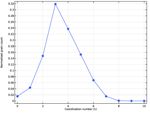
Select the Compute coordination numbers checkbox.
Add Study
1
In the Study toolbar, click  Add Study to open the Add Study window.
2
Go to the Add Study window.
3
Find the Studies subsection. In the Select Study tree, select General Studies > Time Dependent.
4
Click the Add Study button in the window toolbar.
5
In the Study toolbar, click  Add Study to close the Add Study window.
Study 3: Spreading
In the Settings window for Study, type Study 3: Spreading in the Label text field.
Step 1: Time Dependent
1
In the Model Builder window, under Study 3: Spreading click Step 1: Time Dependent.
2
In the Settings window for Time Dependent, locate the Study Settings section.
3
In the Output times text field, type range(t_heap,0.1,t_spread).
4
Locate the Values of Dependent Variables section. Find the Initial values of variables solved for subsection. From the Settings list, choose User controlled.
5
From the Method list, choose Solution.
6
From the Study list, choose Study 2: Heap Formation, Time Dependent.
7
In the Study toolbar, click  Compute.
Results
Grain Positions: Spreading
1
In the Settings window for 3D Plot Group, type Grain Positions: Spreading in the Label text field.
Modify the default plot settings to better visualize the roller rotations.
2
In the Model Builder window, expand the Grain Positions: Spreading node.
Color Expression 1
1
In the Model Builder window, expand the Results > Grain Positions: Spreading > Grain Positions 1 node, then click Color Expression 1.
2
In the Settings window for Color Expression, locate the Expression section.
3
In the Expression text field, type gran.Ng.
4
In the Grain Positions: Spreading toolbar, click  Plot.
Surface 1
1
In the Model Builder window, under Results > Grain Positions: Spreading click Surface 1.
2
In the Settings window for Surface, locate the Coloring and Style section.
3
From the Coloring list, choose Uniform.
4
From the Color list, choose Gray.
Selection 1
1
In the Model Builder window, expand the Surface 1 node, then click Selection 1.
2
In the Settings window for Selection, locate the Selection section.
3
Click to select the  Activate Selection toggle button.
4
5
Click  Remove from Selection.
6
Surface 2
1
In the Model Builder window, under Results > Grain Positions: Spreading right-click Surface 1 and choose Duplicate.
2
In the Settings window for Surface, locate the Coloring and Style section.
3
From the Color list, choose Yellow.
Selection 1
1
In the Model Builder window, expand the Surface 2 node, then click Selection 1.
2
In the Settings window for Selection, locate the Selection section.
3
Click to select the  Activate Selection toggle button.
4
Click  Clear Selection.
5
6
In the Grain Positions: Spreading toolbar, click  Plot.
7
Click the  Zoom Extents button in the Graphics toolbar. The powder bed at the end of the third study should resemble Figure 4.
Spreading
1
In the Grain Positions: Spreading toolbar, click  Animation and choose Player.
2
In the Settings window for Animation, type Spreading in the Label text field.
3
Locate the Frames section. From the Frame selection list, choose All.
4
Click the  Play button in the Graphics toolbar.
1D Histogram
Next, a 1D Histogram of the x-coordinates of the grains is first computed, and the resultant data is used to set up an Interpolation function. This function is then used to compute the packing fraction of the grains within the powder bed.
1
In the Results toolbar, click  1D Plot Group.
2
In the Settings window for 1D Plot Group, type 1D Histogram in the Label text field.
3
Locate the Data section. From the Dataset list, choose Grain 3.
4
From the Time selection list, choose Last.
Histogram 1
1
In the 1D Histogram toolbar, click  Histogram.
2
In the Settings window for Histogram, locate the Expression section.
3
In the Expression text field, type qx.
4
Locate the Bins section. From the Entry method list, choose Limits.
5
In the Limits text field, type range(sample_xmin, sample_width, sample_xmax).
6
Click to expand the Coloring and Style section. Find the Line style subsection. From the Line list, choose None.
7
Find the Line markers subsection. From the Marker list, choose Cycle.
8
In the 1D Histogram toolbar, click  Plot.
9
Right-click Histogram 1 and choose Copy Plot Data to Table.
Definitions
Interpolation 1 (int1)
1
In the Definitions toolbar, click  Interpolation.
2
In the Settings window for Interpolation, locate the Definition section.
3
From the Data source list, choose Result table.
4
Locate the Data Column Settings section. In the Unit text field, type m.
5
Click  Create Plot.
Results
Packing Fraction
1
In the Settings window for 1D Plot Group, click to expand the Title section.
2
From the Title type list, choose None.
3
In the Label text field, type Packing Fraction.
4
Locate the Plot Settings section. Select the x-axis label checkbox.
5
Select the y-axis label checkbox.
6
In the x-axis label text field, type x (m).
7
In the y-axis label text field, type Packing fraction.
Function 1
1
In the Model Builder window, expand the Packing Fraction node, then click Function 1.
2
In the Settings window for Function, locate the y-Axis Data section.
3
In the Expression text field, type int1(x)*pi/6*dg^3/(sample_width*Ly*roller_gap).
4
Locate the x-Axis Data section. Clear the Description checkbox.
5
Locate the Output section. From the Extrapolation list, choose None.
6
In the Packing Fraction toolbar, click  Plot. The plot of the packing fraction in the powder bed as a function of the x-coordinate should resemble Figure 5.
Height Distribution
1
In the Home toolbar, click  Add Plot Group and choose 1D Plot Group.
2
In the Settings window for 1D Plot Group, type Height Distribution in the Label text field.
3
Locate the Data section. From the Dataset list, choose Grain 3.
4
From the Time selection list, choose Last.
5
Locate the Title section. From the Title type list, choose None.
6
Locate the Plot Settings section.
7
Select the x-axis label checkbox. In the associated text field, type qz/dg (1).
8
Select the y-axis label checkbox. In the associated text field, type Normalized grain count.
Histogram 1
1
In the Height Distribution toolbar, click  Histogram.
2
In the Settings window for Histogram, locate the Expression section.
3
In the Expression text field, type qz/dg.
4
Locate the Bins section. From the Entry method list, choose Limits.
5
In the Limits text field, type range(0.05,0.1,roller_gap/dg).
6
Locate the Output section. From the Normalization list, choose Sum of values.
7
Locate the Coloring and Style section. Find the Line markers subsection. From the Marker list, choose Cycle.
8
In the Height Distribution toolbar, click  Plot.
Filter 1
1
In the Height Distribution toolbar, click  Filter.
2
In the Settings window for Filter, locate the Point Selection section.
3
In the Logical expression for inclusion text field, type qx>=sample_xmin && qx<=sample_xmax.
4
In the Height Distribution toolbar, click  Plot. The distribution of the heights of the grains should resemble Figure 6.
Coordination Number Distribution
1
In the Model Builder window, right-click Height Distribution and choose Duplicate.
2
In the Settings window for 1D Plot Group, type Coordination Number Distribution in the Label text field.
3
Locate the Plot Settings section. In the x-axis label text field, type Coordination number (1).
Histogram 1
1
In the Model Builder window, expand the Coordination Number Distribution node, then click Histogram 1.
2
In the Settings window for Histogram, locate the Expression section.
3
In the Expression text field, type gran.Ng.
4
Locate the Bins section. In the Limits text field, type range(-0.5,1.0,10.5).
5
In the Coordination Number Distribution toolbar, click  Plot. The distribution of the grain coordination numbers should resemble Figure 7.