|
|
|
|
1
|
|
2
|
|
3
|
Click Add.
|
|
4
|
Click
|
|
5
|
|
6
|
Click
|
|
1
|
|
2
|
|
3
|
Click
|
|
4
|
Browse to the model’s Application Libraries folder and double-click the file hopper_flow_parameters.txt.
|
|
1
|
|
2
|
|
3
|
|
4
|
|
5
|
|
1
|
|
2
|
|
3
|
|
4
|
|
5
|
|
1
|
|
2
|
Click in the Graphics window and then press Ctrl+A to select both objects.
|
|
3
|
|
4
|
Clear the Keep interior boundaries checkbox.
|
|
1
|
|
2
|
|
1
|
|
2
|
|
3
|
Click to expand the Material Properties section. In the Material properties tree, select Basic Properties > Density.
|
|
4
|
Click
|
|
5
|
|
6
|
Click
|
|
7
|
|
8
|
Click
|
|
9
|
Locate the Material Contents section. In the table, enter the following settings:
|
|
1
|
|
2
|
|
3
|
Locate the Geometric Entity Selection section. From the Geometric entity level list, choose Boundary.
|
|
4
|
|
5
|
Locate the Material Contents section. In the table, enter the following settings:
|
|
1
|
In the Model Builder window, under Component 1 (comp1) > Granular Flow (gran) click Grain Properties 1.
|
|
2
|
|
3
|
|
4
|
|
1
|
In the Model Builder window, under Component 1 (comp1) > Granular Flow (gran) click Contact Between Grains 1.
|
|
2
|
|
3
|
|
4
|
|
5
|
|
6
|
|
7
|
|
1
|
|
2
|
|
3
|
|
4
|
|
5
|
|
6
|
|
7
|
|
1
|
|
3
|
|
4
|
|
5
|
|
6
|
Locate the Released Grain Properties section. In the table, enter the following settings:
|
|
7
|
Locate the Advanced Settings section. In the Number of release attempts per grain text field, type 50 to increase the chances of all the grains being released at each release time.
|
|
1
|
|
1
|
|
2
|
|
3
|
|
4
|
|
5
|
|
6
|
|
7
|
|
8
|
|
1
|
|
2
|
|
1
|
|
2
|
|
3
|
|
4
|
Locate the Physics and Variables Selection section. Select the Modify model configuration for study step checkbox.
|
|
5
|
In the tree, select Component 1 (comp1) > Granular Flow (gran) > Outlet 1 and Component 1 (comp1) > Granular Flow (gran) > Bounding Box 1.
|
|
6
|
Click
|
|
1
|
|
2
|
|
3
|
Click
|
|
5
|
Click
|
|
7
|
|
1
|
|
2
|
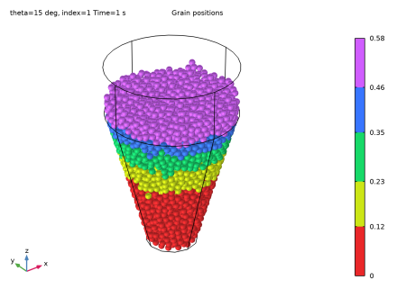
Locate the Data section. From the Parameter value (theta (deg),index) list, choose 1: theta=15 deg, index=1.
|
|
3
|
|
1
|
In the Model Builder window, expand the Results > Grain Positions: Filling > Grain Positions 1 node, then click Color Expression 1.
|
|
2
|
|
3
|
|
4
|
|
5
|
|
6
|
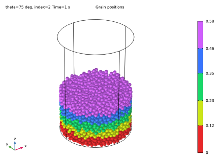
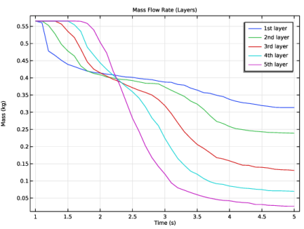
In the Number of bands text field, type 5. The discrete color table with five bands helps in visualizing the grains in the hopper as five distinct layers.
|
|
7
|
|
1
|
|
2
|
|
3
|
|
4
|
|
1
|
|
2
|
|
3
|
|
4
|
Click the
|
|
5
|
Locate the Animation Editing section. From the Parameter value (theta (deg),index) list, choose 2: theta=75 deg, index=2.
|
|
6
|
Click the
|
|
1
|
|
2
|
|
3
|
|
4
|
|
1
|
|
2
|
|
3
|
|
4
|
|
1
|
|
2
|
|
3
|
|
4
|
Locate the Animation Editing section. From the Parameter value (theta (deg),index) list, choose 1: theta=15 deg, index=1.
|
|
5
|
Click the
|
|
6
|
|
7
|
Click the
|
|
1
|
|
2
|
Go to the Add Study window.
|
|
3
|
|
4
|
Click the Add Study button in the window toolbar.
|
|
5
|
|
1
|
|
2
|
|
3
|
|
4
|
Click to expand the Values of Dependent Variables section. Find the Initial values of variables solved for subsection. From the Settings list, choose User controlled.
|
|
5
|
|
6
|
|
7
|
|
8
|
|
9
|
|
1
|
|
2
|
|
3
|
Click
|
|
5
|
Click
|
|
7
|
|
1
|
|
2
|
Locate the Data section. From the Parameter value (theta (deg),index) list, choose 1: theta=15 deg, index=1.
|
|
3
|
|
1
|
In the Model Builder window, expand the Results > Grain Positions: Emptying > Grain Positions 1 node, then click Color Expression 1.
|
|
2
|
|
3
|
|
4
|
|
5
|
|
6
|
|
1
|
|
2
|
|
3
|
|
4
|
|
5
|
|
1
|
|
2
|
|
3
|
|
4
|
Click the
|
|
5
|
Locate the Animation Editing section. From the Parameter value (theta (deg),index) list, choose 2: theta=75 deg, index=2.
|
|
6
|
Click the
|
|
1
|
|
2
|
|
3
|
|
4
|
|
5
|
|
6
|
|
7
|
Locate the Plot Settings section.
|
|
8
|
|
9
|
|
1
|
|
2
|
|
3
|
|
4
|
|
5
|
|
6
|
|
1
|
|
2
|
|
3
|
|
4
|
|
5
|
|
1
|
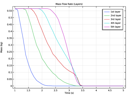
In the Model Builder window, under Results > Mass Flow Rate (Layers) right-click Grain 1 and choose Duplicate.
|
|
2
|
|
3
|
|
1
|
|
2
|
|
3
|
In the Logical expression for inclusion text field, type gran.rti>=6*rel_freq && gran.rti<12*rel_freq.
|
|
1
|
In the Model Builder window, under Results > Mass Flow Rate (Layers) right-click Grain 2 and choose Duplicate.
|
|
2
|
|
3
|
|
1
|
|
2
|
|
3
|
In the Logical expression for inclusion text field, type gran.rti>=12*rel_freq && gran.rti<18*rel_freq.
|
|
1
|
In the Model Builder window, under Results > Mass Flow Rate (Layers) right-click Grain 3 and choose Duplicate.
|
|
2
|
|
3
|
|
1
|
|
2
|
|
3
|
In the Logical expression for inclusion text field, type gran.rti>=18*rel_freq && gran.rti<24*rel_freq.
|
|
1
|
In the Model Builder window, under Results > Mass Flow Rate (Layers) right-click Grain 4 and choose Duplicate.
|
|
2
|
|
3
|
|
1
|
|
2
|
|
3
|
In the Logical expression for inclusion text field, type gran.rti>=24*rel_freq && gran.rti<30*rel_freq.
|
|
4
|
|
1
|
|
2
|
|
3
|
|
4
|
|
1
|
|
2
|
|
3
|
|
4
|
|
5
|
Locate the Plot Settings section.
|
|
6
|
|
7
|
|
1
|
|
2
|
|
3
|
|
4
|
|
5
|
|
7
|