COMSOL 6.4 - Grain Packing

Grain packing refers to the process of packaging grains of differing sizes into a container. Several factors, including the grain shape and size as well as contact forces, can influence the packing efficiency. Furthermore, as the grain size reduces to the scale of millimeters and lower, noncontact forces such as adhesion and van der Waals forces can also greatly influence the packing behavior. Therefore, the prediction of the packing efficiency for a given system of granular material is nontrivial.

This model uses the Granular Flow interface to model the packing behavior of spherical grains of five different diameters. The extent of the packing is characterized by the evaluation of the packing fraction. Three contact force models are used to demonstrate the importance of accurately modeling the contact forces in the packing simulations.

Model Definition

The geometry consists of a rectangular box of equal length and width of 0.2 mm and a height of 0.3 mm. A total of 5000 grains are released into the box and the grain diameters are drawn from a normal distribution with a mean of 10 μm and a standard deviation of 2.5 μm. Periodic boundary conditions are applied along the x and y directions to eliminate the wall effects. The grains are allowed to settle under the influence of gravity and the contact forces for a total of 8 ms. The overall kinetic energy of the grains is tracked to ensure that the resultant bed is stable.

The extent of the packing is characterized by the packing efficiency which is defined as the ratio of the total volume in the sample occupied by the grains divided by the total volume of the sample. The sample under consideration in this model is defined consistently with Ref. 1 and is defined as all the grains located between 30% and 70% of the height of the overall packed bed.

Three contact force models are used to study their effect on the packing efficiency of the grains. The three contact force models are:

•

Hertz–MD which is one of the most common force models used in discrete element method simulations

•

Hertz–MD with adhesion which extends the Hertz–MD model with adhesive (noncontact) forces.

•

Hertz–MD with adhesion and van der Waals forces which extends the previous force model and adds the (noncontact) van der Walls forces between grains that become important when the grain sizes approach the micron scale.

Notes on the COMSOL Implementation

The model is solved using a single study step. After each study step, the solution is stored and the physics settings are modified before running the study step with a different contact force model

The grains are released into the domain using a feature and are allowed to settle under gravity and contact forces. The feature is used in the x and y directions to eliminate wall effects in those directions.

The grain diameters are drawn from a normal distribution with a given mean and standard deviation. In the Granular Flow module, this is achieved by discretizing the continuous normal distribution into discrete bins. Five bins are chosen in this model to represent the discretized normal distribution. The probability calculations for each bin are evaluated as parameters in a feature.

The force computations in the Granular Flow interface rely on sophisticated search algorithms to speed up the simulation times. These algorithms can drastically reduce the number of grains or wall elements that each grain needs to check for contact by only checking the grains or wall elements that lie within a certain search radius of each grain. This search radius is by default equal to the grain radius itself. The search radius needs to be expanded when the contact force models include noncontact forces such as adhesive and van der Waals forces. This expansion of the search radius is controlled by the parameter present in the feature in the Granular Flow Interface. This value can be set to 1.0 for the first contact force model that does not contain any noncontact forces. For the other two contact force models, this value is set to 1.05 to expand the search radius by 5%.

Results and Discussion

Figure 1 shows the packed grains using the Hertz-MD model. The grains are colored by their diameter.

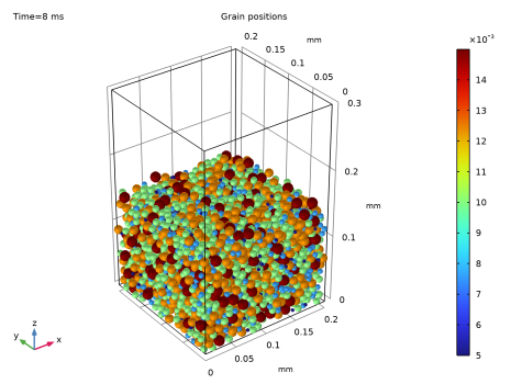
The grains have clearly formed a tightly packed bed.

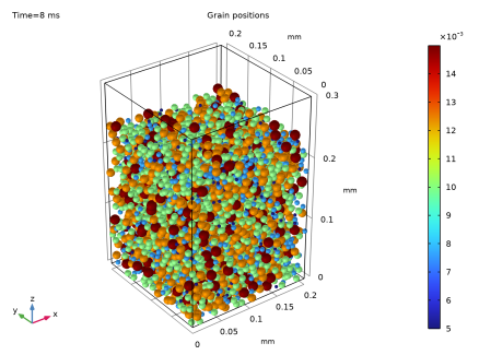
Figure 1: The packed grains using the Hertz–MD model.

The packed grains resulting from the inclusion of the adhesive forces are shown in Figure 2. Figure 3 shows the packed bed resulting from the inclusion of the van der Waals forces. It is evident that the grain packing in these two cases is not as efficient as Figure 1. This is due to the nature of the adhesive forces which can cause grains to be weakly connected to each other even after a collision has taken place.

This decrease in packing efficiency is best visualized in Figure 4 where the packing fractions are plotted as a function of time for all three contact force models. The inclusion of the adhesive forces first reduces the packing fraction, and the inclusion of the van der Waals forces further decreases the packing efficiency.

Finally, Figure 5 shows the evolution of the overall kinetic energy of the grains as a function of time for each of the three contact force models. In all cases, the kinetic energy initially increases as a result of the acceleration due to gravity, and then starts reducing as the repeated collisions dissipate the kinetic energies. However the effect of the adhesive forces can be seen in the reduced dissipation rate of the overall kinetic energies.

Figure 2: The packed grains using the Hertz–MD with adhesion model.

Figure 3: The packed grains using the Hertz–MD with adhesion model with van der Waals forces enabled.

Figure 4: Packing fraction as a function of time.

Figure 5: Average kinetic energy of the grains across the three force models.

Reference

1. E.J. Parteli, J. Schmidt, C. Blümel, K.E. Wirth, W. Peukert, and T. Pöschel, “Attractive particle interaction forces and packing density of fine glass powders,” Sci. Rep., vol. 4, no. 6227, 2014; doi.org/10.1038/srep06227.

Granular_Flow_Module/Flow_and_Material_Characterization/grain_packing

Modeling Instructions

From the menu, choose .

New

In the window, click

Model Wizard

In the window, click

In the tree, select > .

Click .

Click

In the tree, select > .

Click

Global Definitions

Model Parameters

In the window, under click .

In the window for , type Model Parameters in the text field.

Locate the section. Click

Browse to the model’s Application Libraries folder and double-click the file grain_packing_parameters.txt.

Normal Distribution 1 (nd1, nd1_cum, ...)

In the toolbar, click

and choose > .

In the window for , locate the section.

In the text field, type dMean.

In the text field, type delta.

Diameter Distributions

Next, discretize the normal distribution into five bins.

In the toolbar, click

and choose > .

In the window for , type Diameter Distributions in the text field.

Locate the section. In the table, enter the following settings:


Name	Expression	Value	Description
d1	dMean-2*delta	5E-6 m	Diameter, bin 1
d2	dMean-delta	7.5E-6 m	Diameter, bin 2
d3	dMean	1E-5 m	Diameter, bin 3
d4	dMean+delta	1.25E-5 m	Diameter, bin 4
d5	dMean+2*delta	1.5E-5 m	Diameter, bin 5
p1	0.5(delta)(nd1(delta/2+d1)+nd1(d1-delta/2))[1/m]	0.073523	Population, bin 1
p2	0.5(delta)(nd1(delta/2+d2)+nd1(d2-delta/2))[1/m]	0.24079	Population, bin 2
p3	0.5(delta)(nd1(delta/2+d3)+nd1(d3-delta/2))[1/m]	0.35207	Population, bin 3
p4	0.5(delta)(nd1(delta/2+d4)+nd1(d4-delta/2))[1/m]	0.24079	Population, bin 4
p5	0.5(delta)(nd1(delta/2+d5)+nd1(d5-delta/2))[1/m]	0.073523	Population, bin 5

Definitions

Variables 1

In the toolbar, click

and choose .

In the window for , locate the section.

In the table, enter the following settings:


Name	Expression	Unit	Description
zmax	gran.max(if(qz<0.9*Lz,qz,0))	m	Max height
include	if(qz>0.3zmax&&qz<0.7zmax,1,0)		Boolean for inclusion
count	gran.sum(include)		Number of grains included
vol_occ	4pi/3gran.sum(include*gran.rg^3)	m³	Occupied volume
vol_tot	LxLy0.4*zmax	m³	Total volume
pFrac	vol_occ/vol_tot		Packing fraction

Geometry 1

In the window, under click .

In the window for , locate the section.

From the list, choose .

Block 1 (blk1)

In the toolbar, click

In the window for , locate the section.

In the text field, type Lx.

In the text field, type Ly.

In the text field, type Lz.

Click

Materials

Grains

In the toolbar, click

In the window for , type Grains in the text field.

Click to expand the section. In the tree, select > .

Click

In the tree, select > .

Click

In the tree, select > .

Click

Locate the section. In the table, enter the following settings:


Property	Variable	Value	Unit	Property group
Density	rho	rhog	kg/m³	Basic
Poisson’s ratio	nu	pois	1	Basic
Young’s modulus	E	Eg	Pa	Basic

Walls

In the toolbar, click

In the window for , type Walls in the text field.

Locate the section. From the list, choose .

From the list, choose .

Locate the section. In the table, enter the following settings:


Property	Variable	Value	Unit	Property group
Young’s modulus	E	2.5*Eg	Pa	Basic
Poisson’s ratio	nu	pois	1	Basic

Granular Flow (gran)

Grain Properties 1

In the window, under > click .

In the window for , locate the section.

From the list, choose .

Locate the section. In the dg text field, type d1.

Grain Properties 2

In the toolbar, click

and choose .

In the window for , locate the section.

From the list, choose .

Locate the section. In the dg text field, type d2.

Grain Properties 3

Right-click and choose .

In the window for , locate the section.

In the dg text field, type d3.

Grain Properties 4

Right-click and choose .

In the window for , locate the section.

In the dg text field, type d4.

Grain Properties 5

Right-click and choose .

In the window for , locate the section.

In the dg text field, type d5.

Contact Between Grains 1

In the window, click .

In the window for , locate the section.

In the en text field, type en.

In the et text field, type et.

In the μs text field, type mu_s.

In the μr text field, type mu_r.

In the μtw text field, type mu_tw.

Contact with Walls 1

In the window, click .

In the window for , locate the section.

In the en text field, type en.

In the et text field, type et.

In the μs text field, type mu_s.

In the μr text field, type mu_r.

In the μtw text field, type mu_tw.

Release 1

In the toolbar, click

and choose .

Select Domain 1 only.

In the window for , locate the section.

From the list, choose .

In the N text field, type 5000.

In the table, enter the following settings:


Released grain properties	Number fraction of grains
Grain Properties 1	p1
Grain Properties 2	p2
Grain Properties 3	p3
Grain Properties 4	p4
Grain Properties 5	p5