PDF

Angle of Repose
Introduction
When bulk granular materials are poured onto a horizontal surface, they often form a conical heap. The angle of repose is defined as the internal angle that the free surface of the heap forms with the horizontal plane. This angle often depends on a variety of factors including the size and shape of the particles, surface roughness, friction coefficients, and density. The angle of repose is therefore a complex property of the granular system and it is often used in material characterization. Its usefulness is due to the simplicity of its measurement compared to other material or contact properties. It is widely used in many industries such as material storage, conveyors, geotechnical engineering, and pharmaceuticals.
The angle of repose can be evaluated using a number of measurement techniques (Ref. 1) including the hollow cylinder method, fixed funnel method, internal flow funnel method, and rotating drum method. Any of these methods can be chosen based on their relevance in the desired application. This example uses the Granular Flow interface to model the fixed funnel method, where a funnel is kept at a fixed height. The funnel is first filled with grains which are subsequently released and collected as a heap. The resultant heap is then analyzed using Model Methods to evaluate the angle of repose.
Model Definition
The geometry consists of a hopper surrounded by a rectangular box. A total of 5000 grains of diameter 20 mm are directly released into the hopper and are allowed to settle under gravity. The grains are then allowed to exit the hopper through its outlet and are collected on the horizontal surface of the box. The model geometry is shown in Figure 1.
Once the grain heap stabilizes, the grain positions are used to compute the angle of repose using the following algorithm as described in Ref. 1.
1
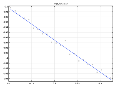
The grain positions are projected onto the xz-plane to form a 2D representation of the heap.
2
3
4
Figure 1: Model geometry.
Notes on the COMSOL Implementation
The model is solved using two studies. In the first study, the grains are released into the hopper using a Release feature to release the grains which are then allowed to settle under gravity. The degrees of freedom of the grains at the end of this study are used to initialize the second study in which the Outlet feature is used to simulate the discharge of the grains.
Once the second study is completed, the computation of the angle of repose is achieved by adding and running a Model Method.
Note: Model methods can only be set up in the COMSOL Desktop environment on the Windows version of COMSOL Multiphysics.
Results and Discussion
The grain positions at the end of the first study are shown in Figure 2 and are colored by their speed in m/s.
Figure 2: Hopper filled with grains. The grains are colored based on their speeds in m/s.
The grain positions at the end of the second study are shown in Figure 3 and are again colored by their speed in m/s. The grains form a symmetrical heap on the horizontal surface. The speeds of the grains in the heap are again very low thus indicating that the grains have formed a stable heap.
The outline of the right and left sections of the free surface, along with their least-squares fit are shown in Figure 4 and Figure 5, respectively. The least-squares fit obtained for each section shows that the heap’s outline is fairly linear and the average angle of repose can be evaluated from the slopes.
Figure 3: Heap of grains formed after emptying the hopper. The grains are colored by their speed in m/s.
Figure 4: Outline and the linear fit for the right section of the heap.
Figure 5: Outline and the linear fit for the left section of the heap.
Reference
1. D. Müller, E. Fimbinger, and C. Brand, “Algorithm for the determination of the angle of repose in bulk material analysis,” Powder Technology, vol. 383, pp. 598–605, 2021.
Application Library path: Granular_Flow_Module/Flow_and_Material_Characterization/angle_of_repose
Modeling Instructions
From the Main Toolbar menu, choose New.
New
In the New window, click  Model Wizard.
Model Wizard
1
In the Model Wizard window, click  3D.
2
In the Select Physics tree, select Fluid Flow > Granular Flow (gran).
3
Click Add.
4
Click  Study.
5
In the Select Study tree, select General Studies > Time Dependent.
6
Global Definitions
Model Parameters
1
In the Model Builder window, under Global Definitions click Parameters 1.
2
In the Settings window for Parameters, type Model Parameters in the Label text field.
3
Locate the Parameters section. Click  Load from File.
4
Geometry 1
Cylinder 1 (cyl1)
1
In the Geometry toolbar, click  Cylinder.
2
In the Settings window for Cylinder, locate the Size and Shape section.
3
In the Radius text field, type D_in/2.
4
In the Height text field, type H_cyl.
Cone 1 (cone1)
1
In the Geometry toolbar, click  Cone.
2
In the Settings window for Cone, locate the Size and Shape section.
3
In the Bottom radius text field, type D_out/2.
4
In the Height text field, type H_cone.
5
In the Top radius text field, type D_in/2.
6
Locate the Position section. In the z text field, type -H_cone.
Block 1 (blk1)
1
In the Geometry toolbar, click  Block.
2
In the Settings window for Block, locate the Size and Shape section.
3
In the Width text field, type L_plate.
4
In the Depth text field, type L_plate.
5
In the Height text field, type H_fall+H_cyl+H_cone.
6
Locate the Position section. In the x text field, type -L_plate/2.
7
In the y text field, type -L_plate/2.
8
In the z text field, type -H_fall-H_cone.
9
Click  Build All Objects.
10
Click the  Zoom Extents button in the Graphics toolbar.
11
Click the  Transparency button in the Graphics toolbar.
Ignore Faces 1 (igf1)
1
In the Geometry toolbar, click  Virtual Operations and choose Ignore Faces.
2
On the object fin, select Boundary 10 only.
3
In the Geometry toolbar, click  Build All. The geometry should look like Figure 1.
Add Material
1
In the Materials toolbar, click  Add Material to open the Add Material window.
2
Go to the Add Material window.
3
In the tree, select Built-in > Steel AISI 4340.
4
Click the Add to Component button in the window toolbar.
5
In the Materials toolbar, click  Add Material to close the Add Material window.
Materials
Steel AISI 4340 (mat1)
1
In the Settings window for Material, locate the Geometric Entity Selection section.
2
From the Geometric entity level list, choose Boundary.
3
From the Selection list, choose All boundaries.
Granular Flow (gran)
Grain Properties 1
1
In the Model Builder window, under Component 1 (comp1) > Granular Flow (gran) click Grain Properties 1.
2
In the Settings window for Grain Properties, locate the Granular Material Properties section.
3
From the ρg list, choose User defined. In the associated text field, type rho.
4
From the Eg list, choose User defined. In the associated text field, type E.
5
From the νg list, choose User defined. In the associated text field, type pois.
6
Locate the Size section. In the dg text field, type dg.
Contact Between Grains 1
1
In the Model Builder window, click Contact Between Grains 1.
2
In the Settings window for Contact Between Grains, locate the Contact Properties section.
3
In the en text field, type 0.4.
4
In the et text field, type 0.5.
5
In the μs text field, type 0.8.
6
In the μr text field, type 0.4.
7
In the μtw text field, type 0.4.
Contact with Walls 1
1
In the Model Builder window, click Contact with Walls 1.
2
In the Settings window for Contact with Walls, locate the Contact Properties section.
3
In the en text field, type 0.3.
4
In the et text field, type 0.5.
5
In the μs text field, type 0.7.
6
In the μr text field, type 0.6.
7
In the μtw text field, type 0.55.
Release 1
1
In the Physics toolbar, click  Domains and choose Release.
2
3
In the Settings window for Release, locate the Released Grain Properties section.
4
Outlet 1
1
In the Physics toolbar, click  Boundaries and choose Outlet.
2
3
Click the  Transparency button in the Graphics toolbar.
Grain Packing
1
In the Model Builder window, click Study 1.
2
In the Settings window for Study, type Grain Packing in the Label text field.
Step 1: Time Dependent
1
In the Model Builder window, under Grain Packing click Step 1: Time Dependent.
2
In the Settings window for Time Dependent, locate the Study Settings section.
3
In the Output times text field, type range(0,0.1,t_fill).
4
Locate the Physics and Variables Selection section. Select the Modify model configuration for study step checkbox.
5
In the tree, select Component 1 (comp1) > Granular Flow (gran) > Outlet 1.
6
Click  Disable.
7
In the Study toolbar, click  Compute.
Results
Grain Positions 1
The grain positions at the end of the Grain Packing study should resemble Figure 2. Now, add another study to simulate the emptying of the hopper and the grain heap formation.
1
From the Home menu, choose Add Study.
Add Study
1
Go to the Add Study window.
2
Find the Studies subsection. In the Select Study tree, select General Studies > Time Dependent.
3
Click the Add Study button in the window toolbar.
4
From the Home menu, choose Add Study.
Emptying
In the Settings window for Study, type Emptying in the Label text field.
Step 1: Time Dependent
1
In the Model Builder window, expand the Grain Positions (gran) node, then click Emptying > Step 1: Time Dependent.
2
In the Settings window for Time Dependent, locate the Study Settings section.
3
In the Output times text field, type range(t_fill,0.1,t_fill+t_empty).
4
Click to expand the Values of Dependent Variables section. Find the Initial values of variables solved for subsection. From the Settings list, choose User controlled.
5
From the Method list, choose Solution.
6
From the Study list, choose Grain Packing, Time Dependent.
7
In the Study toolbar, click  Compute.
Results
Animation 1
1
In the Grain Positions (gran) 1 toolbar, click  Animation and choose Player.
2
In the Settings window for Animation, locate the Frames section.
3
From the Frame selection list, choose All.
4
Click the  Play button in the Graphics toolbar. This plays the animation of the grains emptying from the hopper and forming a heap.
Grain Positions (gran) 1
Click the  Go to XZ View button in the Graphics toolbar. The heap of grains formed should resemble Figure 3.
Application Builder
The angle of repose can be computed using an Application Method. These may be added to an existing model via a Model Method using the Application Builder. Note that the Application Builder is only available in the Windows® version of the COMSOL Desktop. But once the Model Method is created, it can be run in both the Linux and Mac versions.
In the Home toolbar, click  Application Builder.
Methods
The code for the computing and plotting the angle of repose can be simplified by using utility classes.
util1
1
In the Home toolbar, click  More Libraries and choose Utility Class.
2
In the Application Builder window, right-click util1 and choose Edit.
3
Copy the code for the utilities createGrainEval and createLsqFitTables and paste it into the Utility Class editor for util1.
// Create the Grain evaluations
    public static NumericalFeature createGrainEval(String tag, String data, String level, NumericalFeatureList numericalList) {
       NumericalFeature grn;
     if (numericalList.index(tag) == -1)
       grn = model.result().numerical().create(tag, "Grain");
     else
       grn = numericalList.get(tag);
     grn.setIndex("looplevelinput", level, 0);
     grn.set("data", data);
     return grn;
   }
   
 // Create the Least Squares Fit Table
 public static FunctionFeature createLsqFitTables(String miList, String miTag, double[][] data) {
   FunctionFeatureList functionList = model.func();
   FunctionFeature functionFeature;
   
   if (functionList.index(miList) == -1) {
     functionFeature = functionList.create(miList, "LeastSquares");
     functionFeature.label(miTag);
     with(functionFeature);
       setEntry("columnType", "col2", "value");
     endwith();
   }
   else {
     functionFeature = functionList.get(miList);
   }
   
   with(functionFeature);
     for (int k = 0; k < data.length; k++) {
       setIndex("table", data[k][0], k, 0);
       setIndex("table", data[k][1], k, 1);
     }
   endwith();
   return functionFeature;
 }
Global Method
Now add a Model Method to compute the angle of repose that uses the utility functions.
1
In the Home toolbar, click New Method and choose Global Method.
2
In the Global Method dialog, type computeAOR in the Name text field.
3
computeAOR
1
In the Application Builder window, under Methods click computeAOR.
2
Copy the code for method computeAOR and paste it into the Method editor.
ModelNode comp = getCurrentComponent();
 GeomSequence geom = comp.geom(comp.geom().tags()[0]);
 if (geom.getSDim() != 3) {
   error("The model does not have a 3D geometry.");
 }
 
 // Get the grain positions
 NumericalFeatureList numericalList = model.result().numerical();
 NumericalFeature grn1 = util1.createGrainEval("grn1", "gran2", "last", numericalList);
 NumericalFeature grn2 = util1.createGrainEval("grn2", "gran2", "last", numericalList);
 NumericalFeature grn3 = util1.createGrainEval("grn3", "gran2", "last", numericalList);
 
 grn1.set("expr", "qx");
 grn2.set("expr", "qz");
 grn3.set("expr", "gran.rg");
 
 double[][] out1 = grn1.getReal();
 double[][] out2 = grn2.getReal();
 double[][] out3 = grn3.getReal();
 
 double[] qx = transpose(out1)[0];
 double[] qz = transpose(out2)[0];
 double[] rad = transpose(out3)[0];
 
 int numGrains = out1.length;
 
 // Get the 2D projection onto the x-z plane and divide it into bins
 double xMin = java.util.Arrays.stream(qx).min().getAsDouble();
 double xMax = java.util.Arrays.stream(qx).max().getAsDouble();
 double rMin = java.util.Arrays.stream(rad).max().getAsDouble();
 
 // Calculate the bin info
 int numBins = (int) Math.ceil((xMax-xMin)/rMin);
 double binSize = (xMax-xMin)/numBins;
 
 // Calculate the height of each bin
 java.util.ArrayList<Double> binHeights = new java.util.ArrayList<>();
 for (int i = 0; i < numBins; i++)
   binHeights.add(Double.NEGATIVE_INFINITY);
 
 int idx;
 for (int i = 0; i < numGrains; i++) {
   idx = (int) Math.floor((qx[i]-xMin)/binSize);
   idx = Math.min(idx, numBins-1);
   binHeights.set(idx, Math.max(binHeights.get(idx), qz[i]));
 }
 
 // Clean the image (Remove grains not in pile)
 int upperIdx = numBins;
 int lowerIdx = -1;
 
 // Identify the bin with the maximum height
 double maxHeight = java.util.Arrays.stream(qz).max().getAsDouble();
 idx = Math.min(binHeights.indexOf(maxHeight), numBins-1);
 
 // Fan out in both directions to find any empty bins
 for (int i = idx; i < numBins; i++) {
   if (binHeights.get(i) == Double.NEGATIVE_INFINITY) {
     upperIdx = i;
     break;
   }
 }
 for (int i = idx; i >= 0; i--) {
   if (binHeights.get(i) == Double.NEGATIVE_INFINITY) {
     lowerIdx = i;
     break;
   }
 }
 
 // Remove the grains outside the limits
 for (int i = numBins-1; i >= upperIdx; i--)
   binHeights.remove(i);
 for (int i = lowerIdx; i >= 0; i--)
   binHeights.remove(i);
 
 // Get the outline
 xMin += Math.max(0, lowerIdx)*binSize;
 xMax -= Math.max(numBins-upperIdx, 0)*binSize;
 numBins = binHeights.size();
 
 double[][] outline = new double[numBins][2];
 for (int i = 0; i < numBins; i++) {
   outline[i][0] = binSize*(i+1)-0.5*(xMax-xMin);
   outline[i][1] = binHeights.get(i);
 }
 
 // Get the slopes of the 2 sections
 int sidx, eidx, midx;
 midx = (int) numBins/2;
 
 // Right section
 sidx = (int) midx+midx/4;
 eidx = (int) midx+3*midx/4;
 
 double[][] dataRight = new double[eidx-sidx+1][2];
 for (int i = 0; i < dataRight.length; i++) {
   dataRight[i][0] = outline[sidx+i][0];
   dataRight[i][1] = outline[sidx+i][1];
 }
 
 FunctionFeature sec1 = util1.createLsqFitTables("lsq1", "Right Section", dataRight);
 sec1.run();
 double m1 = sec1.getDouble("plist", 1);
 double ang1 = Math.toDegrees(Math.atan(Math.abs(m1)));
 
 sidx = (int) midx/4;
 eidx = (int) midx-1*midx/4;
 
 double[][] dataLeft = new double[eidx-sidx+1][2];
 for (int i = 0; i < dataLeft.length; i++) {
   dataLeft[i][0] = outline[sidx+i][0];
   dataLeft[i][1] = outline[sidx+i][1];
 }
 FunctionFeature sec2 = util1.createLsqFitTables("lsq2", "Left Section", dataLeft);
 sec2.run();
 double m2 = sec2.getDouble("plist", 1);
 double ang2 = Math.toDegrees(Math.atan(Math.abs(m2)));
 double avgAOR = 0.5*(ang1+ang2);
 message("Angle of repose = "+avgAOR);
Methods
1
In the Home toolbar, click  Model Builder to switch to the main desktop.
Add a Method Call to computeAOR in order to run it.
2
In the Developer toolbar, click  Method Call and choose computeAOR.
Global Definitions
Compute Angle of Repose
1
In the Model Builder window, under Global Definitions click ComputeAOR 1.
2
In the Settings window for Method Call, type Compute Angle of Repose in the Label text field.
3
Click  Run. Click Yes if the Confirm Run Method dialogue box appears.
The computeAOR method projects the grains onto the x-z plane and picks out the approximate outline of the heap on this projection. It then divides the outline into a left section and a right section. For each section, a portion of the data points are used to determine the line of best fit in order to estimate the slopes. These two slopes are converted to angles and the average value is displayed as an output in the Messages window.
Right Section (lsq1_fun1)
The data corresponding to the central half portion of the outline for the right section is visible in the Data section, and the slope is given by the a1 parameter as seen in the Parameters section.
1
In the Model Builder window, under Global Definitions click Right Section (lsq1_fun1).
2
In the Settings window for Least-Squares Fit, click  Create Plot.
Results
1D Plot Group 3
The plot should resemble Figure 4.
Global Definitions
Left Section (lsq2_fun1)
Similarly, the data corresponding to the left section is visible in the Data section, and the slope is given by the a1 parameter as seen in the Parameters section.
1
In the Model Builder window, under Global Definitions click Left Section (lsq2_fun1).
2
In the Settings window for Least-Squares Fit, click  Create Plot.
Results
1D Plot Group 4
The plot should resemble Figure 5.