|
|
|
|
•
|
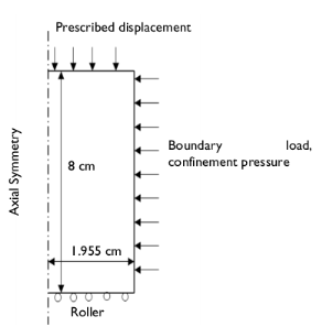
Density ρ = 2400 kg/m3, Poisson’s ratio ν = 0.35, slope of critical state line M = 1.2, swelling index κ = 0.02, compression index λ = 0.1, void ratio eref = 1 at a reference pressure pref = 98 kPa, and initial consolidation pressure pc0 = 100 kPa or 500 kPa.
|
|
•
|
|
1
|
|
2
|
|
3
|
Click Add.
|
|
4
|
Click
|
|
5
|
|
6
|
Click
|
|
1
|
|
2
|
|
1
|
In the Model Builder window, under Component 1 (comp1) right-click Definitions and choose Variables.
|
|
2
|
|
1
|
|
2
|
|
3
|
|
4
|
|
5
|
Click
|
|
1
|
|
2
|
In the Settings window for Elastoplastic Soil Material, type Modified Cam-Clay Material Model in the Label text field.
|
|
4
|
Locate the Elastoplastic Soil Material section. Find the Parameters subsection. From the M list, choose From material.
|
|
5
|
|
6
|
|
7
|
|
8
|
|
1
|
|
2
|
In the Settings window for External Stress, type External Stress [Triaxial Test] in the Label text field.
|
|
3
|
|
4
|
|
1
|
|
1
|
|
3
|
|
4
|
|
5
|
|
1
|
|
1
|
|
3
|
|
4
|
|
5
|
|
1
|
In the Model Builder window, under Component 1 (comp1) > Solid Mechanics (solid), Ctrl-click to select Roller 1 and Prescribed Displacement 1.
|
|
2
|
Right-click and choose Group.
|
|
1
|
In the Model Builder window, under Component 1 (comp1) > Solid Mechanics (solid), Ctrl-click to select Roller 2 and Boundary Load 1.
|
|
2
|
Right-click and choose Group.
|
|
1
|
In the Model Builder window, under Component 1 (comp1) right-click Materials and choose Blank Material.
|
|
2
|
|
3
|
Locate the Material Contents section. In the table, enter the following settings:
|
|
1
|
|
2
|
|
3
|
|
4
|
|
5
|
Click
|
|
1
|
|
2
|
|
3
|
|
1
|
|
2
|
|
3
|
Select the Modify model configuration for study step checkbox.
|
|
4
|
|
5
|
Right-click and choose Disable.
|
|
6
|
|
7
|
Click
|
|
1
|
|
2
|
|
3
|
Click
|
|
5
|
|
1
|
|
2
|
Go to the Add Study window.
|
|
3
|
|
4
|
Click the Add Study button in the window toolbar.
|
|
5
|
|
1
|
|
2
|
Clear the Generate default plots checkbox.
|
|
3
|
|
4
|
|
1
|
|
2
|
Click
|
|
1
|
|
2
|
|
3
|
Select the Modify model configuration for study step checkbox.
|
|
4
|
In the tree, select Component 1 (comp1) > Solid Mechanics (solid) > Modified Cam-Clay Material Model > External Stress [Triaxial Test] and Component 1 (comp1) > Solid Mechanics (solid) > Triaxial Test.
|
|
5
|
Right-click and choose Disable.
|
|
6
|
|
7
|
Click
|
|
9
|
|
1
|
|
2
|
|
3
|
Click
|
|
4
|
|
5
|
Click OK.
|
|
6
|
|
8
|
Select the Apply conversions to expressions with the same dimensions checkbox.
|
|
9
|
Click
|
|
1
|
|
2
|
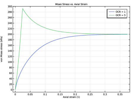
In the Settings window for 1D Plot Group, type Mises Stress vs. Axial Strain in the Label text field.
|
|
3
|
|
4
|
|
5
|
Locate the Plot Settings section.
|
|
6
|
|
7
|
|
1
|
|
2
|
|
3
|
|
4
|
|
6
|
|
7
|
|
8
|
|
9
|
|
10
|
|
1
|
|
2
|
|
3
|
|
4
|
Locate the Legends section. In the table, enter the following settings:
|
|
5
|
|
1
|
|
2
|
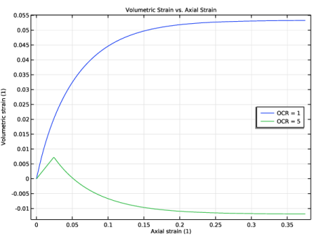
In the Settings window for 1D Plot Group, type Volumetric Strain vs. Axial Strain in the Label text field.
|
|
3
|
|
4
|
|
5
|
Locate the Plot Settings section.
|
|
6
|
|
7
|
|
8
|
|
1
|
|
2
|
|
3
|
|
4
|
|
6
|
|
7
|
|
8
|
|
9
|
|
10
|
|
1
|
|
2
|
|
3
|
|
5
|
Locate the Legends section. In the table, enter the following settings:
|
|
6
|
|
1
|
|
2
|
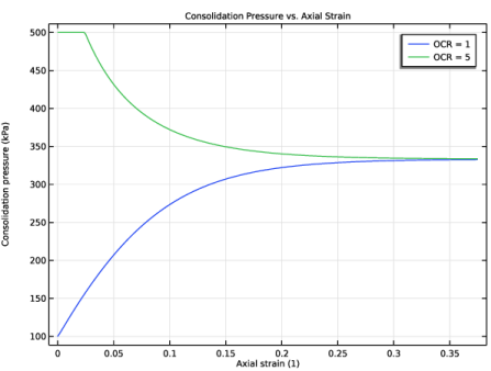
In the Settings window for 1D Plot Group, type Consolidation Pressure vs. Axial Strain in the Label text field.
|
|
3
|
|
4
|
|
5
|
Locate the Plot Settings section.
|
|
6
|
|
7
|
|
1
|
|
2
|
|
3
|
|
4
|
|
6
|
Click Replace Expression in the upper-right corner of the y-Axis Data section. From the menu, choose Component 1 (comp1) > Solid Mechanics > Soil material properties > Modified Cam-clay > solid.epm1.pc - Consolidation pressure - Pa.
|
|
7
|
|
8
|
|
9
|
|
10
|
|
1
|
|
2
|
|
3
|
|
5
|
Locate the Legends section. In the table, enter the following settings:
|
|
6
|
|
1
|
|
2
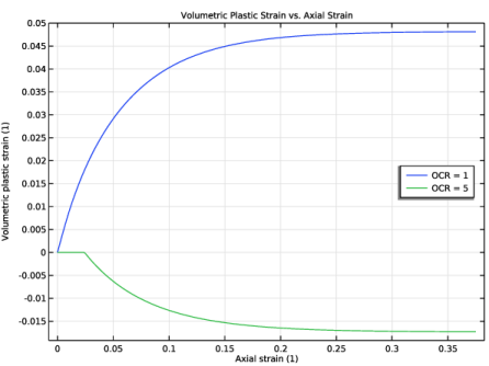
|
In the Settings window for 1D Plot Group, type Volumetric Plastic Strain vs. Axial Strain in the Label text field.
|
|
3
|
|
4
|
|
5
|
Locate the Plot Settings section.
|
|
6
|
|
7
|
|
8
|
|
1
|
|
2
|
|
3
|
|
4
|
|
6
|
|
7
|
|
8
|
|
9
|
|
10
|
|
1
|
|
2
|
|
3
|
|
5
|
Locate the Legends section. In the table, enter the following settings:
|
|
6
|
|
1
|
|
2
|
|
3
|
Locate the Data section. From the Dataset list, choose Study: Oedometer Test/Parametric Solutions 2 (sol6).
|
|
4
|
|
5
|
|
6
|
Locate the Plot Settings section.
|
|
7
|
|
8
|
|
9
|
|
1
|
|
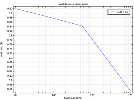
3
|
In the Settings window for Point Graph, click Replace Expression in the upper-right corner of the y-Axis Data section. From the menu, choose Component 1 (comp1) > Solid Mechanics > Soil material properties > Modified Cam-clay > solid.epm1.evoid - Void ratio - 1.
|
|
4
|
|
5
|
|
6
|
|
7
|
|
9
|
|
1
|
|
2
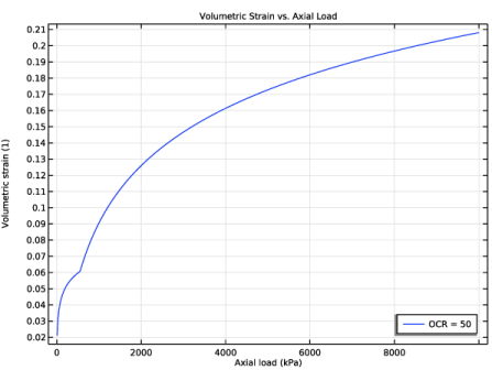
|
In the Settings window for 1D Plot Group, type Volumetric Strain vs. Axial Load in the Label text field.
|
|
3
|
Locate the Data section. From the Dataset list, choose Study: Oedometer Test/Parametric Solutions 2 (sol6).
|
|
4
|
|
5
|
|
6
|
Locate the Plot Settings section.
|
|
7
|
|
8
|
|
9
|
|
1
|
|
3
|
|
4
|
|
5
|
|
6
|
|
7
|
|
8
|
|
10
|
|
1
|
In the Model Builder window, under Results, Ctrl-click to select Mises Stress vs. Axial Strain, Volumetric Strain vs. Axial Strain, Consolidation Pressure vs. Axial Strain, and Volumetric Plastic Strain vs. Axial Strain.
|
|
2
|
Right-click and choose Group.
|
|
1
|
In the Model Builder window, under Results, Ctrl-click to select Void Ratio vs. Axial Load and Volumetric Strain vs. Axial Load.
|
|
2
|
Right-click and choose Group.
|