PDF

Triaxial and Oedometer Test with Hardening Soil Material Model
Introduction
In this example, triaxial and oedometer tests on a cylindrical soil sample are simulated using a Hardening Soil material model.
The triaxial test consists of two stages: an initial isotropic compression is followed by an axial compression. The oedometer test only have an axial compression stage. The analysis can be simplified by taking the axial symmetry of the specimen into account. The results are compared with those presented in Ref. 1 and Ref. 2.
The expected hyperbolic stress–strain relation is recovered by the model. It is also verified that the asymptotic value of the axial stress is equal to the analytical value of the failure stress. In the oedometer test, loading and unloading cycles are conducted to assess the robustness of the numerical implementation.
Model Definition
In this example, a cylindrical soil specimen of 10 cm in diameter and height is loaded as shown in Figure 1.
For the triaxial test, a confinement pressure is applied to create a state of isotropic compression. Thereafter, the soil sample is compressed axially.
For the oedometer test, the soil sample is compressed axially and constrained on the side.
Figure 1: Dimensions, boundary conditions, and boundary loads for the triaxial test.
Soil Properties
The soil properties for loose Hostun sand are inspired from Ref. 1 and Ref. 2. Along with some properties given in the references, the material parameters are presented in Table 1.
ν
ρ
Eiref
Eurref
ϕ
ψ
Rf
e0
pref
Kc
pcc0
pc0
Constraints and Loads
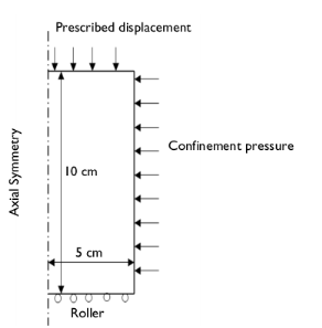
For the triaxial test, a confinement pressure of 300 kPa is applied using the In situ stress option in the External Stress node to model the isotropic compression step. For axial compression, the soil sample is compressed by applying a prescribed displacement on the top boundary. Allow the top boundary to expand freely in the radial direction and apply a roller boundary condition on the bottom boundary.
Results and Discussion
The analytical solution to the axial failure stress for the triaxial test is given by the Mohr–Coulomb criterion
(1)
The axial failure stress in compression is given by
The values of the axial failure stress are shown in Table 2.
σ1
For the sake of consistency with the geomechanical convention, the compressive axial stress and axial strain are plotted along the positive axis in all figures.
The axial stress versus axial strain curves for the triaxial test are shown in Figure 2. The stress–strain curve has an hyperbolic shape, which is a characteristic of the Hardening Soil material model; as the axial displacement increases, the axial stress increases hyperbolically and approaches the failure stress given in Table 2. The results presented for the axial compression case in Figure 2 also closely match the results presented in Ref. 1 (see Figure 6 therein).
The same behavior is observed for the von Mises stress in axial compression; it asymptotically matches the ultimate deviatoric stress based on the Mohr–Coulomb criterion; see Figure 3. The results presented for the axial compression case in Figure 3 also closely match the results presented in Ref. 2 (see Figure 12 therein). The shear failure stress is reached at a compressive axial strain of 0.11, which is similar to the value reported in Ref. 2.
Figure 2: Axial stress versus axial strain for the triaxial test.
.
Figure 3: von Mises stress versus axial strain for the triaxial test.
Figure 4 shows the variations in volumetric strain versus applied axial strain. The volumetric strain shows parabolic behavior with respect to the axial strain, as shown in Ref. 2 (see Figure 13 therein). The volumetric strain matches well with the result presented in the Ref. 1. The volumetric strain is highly dependent on the mobilized dilatation angle formulation.
The dilatancy characteristics of a soil describes its volumetric response to shearing. For the Hardening Soil model presented in Ref. 1, Rowe’s stress dilatancy theory is used, where the mobilized dilatancy angle, ψm, is related to the critical state friction angle, ϕc, and the mobilized friction angle, ϕm:
(2)
The authors in Ref. 2 use the modified Rowe’s formulation which is written as:
(3)
This example uses Rowe’s formulation (similar to Ref. 1), which gives a linear distribution with respect to the mobilized friction angle. The result is shown in Figure 6.
Figure 4: Volumetric strain versus axial strain in the triaxial test.
Figure 5: Mobilized dilatancy angle versus mobilized friction angle in the triaxial test.
The axial stress versus axial strain curves in the cyclic oedometer test are shown in Figure 6. The stress–strain curves for four different loading-unloading cycles presented in Figure 6 also match the results presented in Ref. 2 (see Figure 7 therein). Figure 7 shows the linear variation in volumetric strain with applied axial strain.
Figure 6: Axial stress versus axial strain in the oedometer test.
Figure 7: Volumetric strain versus axial strain in the oedometer test.
Notes About the COMSOL Implementation
The in situ stress is the stress in the soil sample represented in the strain-free configuration. There are two methods to account for in situ stresses in COMSOL Multiphysics. One method is to create two stationary study steps or studies, using a combination of Initial Stress and Strain and External Stress nodes. The second method is to use the In situ stress option in the External Stress node, which gives initial stresses in the soil sample without any strain. In this example, the second method is used to model the in situ stress in the soil samples.
References
1. T. Schanz, P.A. Vermeer, and P.G. Bonnier, “The Hardening Soil Model: Formulation and Verification,” Beyond 2000 in Computational Geotechnics, Rotterdam, 1999.
2. T.A. Bower, P.J. Cleall, and A.D. Jefferson, “A Reformulated Hardening Soil Model,” Proceedings of the Institution of Civil Engineers — Engineering and Computational Mechanics, vol. 173, no. 1, pp. 11–29, 2020.
3. T. Forrister, “Analyzing Triaxial Testing Methods for Geomechanics,” COMSOL Blog, 5 Mar. 2018, www.comsol.com/blogs/analyzing-triaxial-testing-methods-for-geomechanics/.
Application Library path: Geomechanics_Module/Verification_Examples/triaxial_and_oedometer_test_hs
Modeling Instructions
From the File menu, choose New.
New
In the New window, click  Model Wizard.
Model Wizard
1
In the Model Wizard window, click  2D Axisymmetric.
2
In the Select Physics tree, select Structural Mechanics > Solid Mechanics (solid).
3
Click Add.
4
Click  Study.
5
In the Select Study tree, select General Studies > Stationary.
6
Global Definitions
Parameters 1
1
In the Model Builder window, under Global Definitions click Parameters 1.
2
In the Settings window for Parameters, locate the Parameters section.
3
Click  Load from File.
4
Pressure
1
In the Home toolbar, click  Functions and choose Global > Interpolation.
2
In the Settings window for Interpolation, type Pressure in the Label text field.
3
Locate the Definition section. In the Function name text field, type P.
4
5
Locate the Units section. In the Argument table, enter the following settings:
6
In the Function table, enter the following settings:
Define variables for the failure stress in axial compression based on the Mohr–Coulomb criterion.
Definitions
Variables 1
1
In the Model Builder window, under Component 1 (comp1) right-click Definitions and choose Variables.
2
In the Settings window for Variables, locate the Variables section.
3
Geometry 1
Rectangle 1 (r1)
1
In the Geometry toolbar, click  Rectangle.
2
In the Settings window for Rectangle, locate the Size and Shape section.
3
In the Width text field, type 5[cm].
4
In the Height text field, type 10[cm].
5
Click  Build Selected.
6
Click  Build Selected.
7
Click the  Zoom Extents button in the Graphics toolbar.
Solid Mechanics (solid)
Hardening Soil
1
In the Physics toolbar, click  Domains and choose Elastoplastic Soil Material.
2
In the Settings window for Elastoplastic Soil Material, type Hardening Soil in the Label text field.
3
4
Locate the Elastoplastic Soil Material section. From the Material model list, choose Hardening soil.
5
From the ψm list, choose Rowe.
6
Find the Parameters subsection. From the Eiref list, choose From material.
7
In the Rf text field, type 0.95.
Apply a confinement pressure of 300 kPa using an External Stress node.
External Stress 1
1
In the Physics toolbar, click  Attributes and choose External Stress.
2
In the Settings window for External Stress, locate the External Stress section.
3
From the Stress input list, choose In situ stress.
4
In the σins text field, type -p0.
Add a Cap and Cutoff node.
Hardening Soil
In the Model Builder window, click Hardening Soil.
Cap and Cutoff 1
In the Physics toolbar, click  Attributes and choose Cap and Cutoff.
Roller 1
1
In the Physics toolbar, click  Boundaries and choose Roller.
2
Prescribed Displacement 1
1
In the Physics toolbar, click  Boundaries and choose Prescribed Displacement.
2
3
In the Settings window for Prescribed Displacement, locate the Prescribed Displacement section.
4
From the Displacement in z direction list, choose Prescribed.
5
In the u0z text field, type disp.
Roller 2
1
In the Physics toolbar, click  Boundaries and choose Roller.
2
Boundary Load 1
1
In the Physics toolbar, click  Boundaries and choose Boundary Load.
2
3
In the Settings window for Boundary Load, locate the Force section.
4
From the Load type list, choose Pressure.
5
In the p text field, type P(para).
Prescribed Displacement 1, Roller 1
1
In the Model Builder window, under Component 1 (comp1) > Solid Mechanics (solid), Ctrl-click to select Roller 1 and Prescribed Displacement 1.
2
Triaxial Test
In the Settings window for Group, type Triaxial Test in the Label text field.
Boundary Load 1, Roller 2
1
In the Model Builder window, under Component 1 (comp1) > Solid Mechanics (solid), Ctrl-click to select Roller 2 and Boundary Load 1.
2
Oedometer Test
In the Settings window for Group, type Oedometer Test in the Label text field.
Materials
Soil Material
1
In the Model Builder window, under Component 1 (comp1) right-click Materials and choose Blank Material.
2
In the Settings window for Material, type Soil Material in the Label text field.
3
Locate the Material Contents section. In the table, enter the following settings:
One mesh element is sufficient for this analysis.
Mesh 1
Mapped 1
In the Mesh toolbar, click  Mapped.
Distribution 1
1
Right-click Mapped 1 and choose Distribution.
2
In the Settings window for Distribution, locate the Boundary Selection section.
3
From the Selection list, choose All boundaries.
4
Locate the Distribution section. In the Number of elements text field, type 1.
5
Click  Build Selected.
Study: Triaxial Test
Disable the default plots for this study.
1
In the Model Builder window, click Study 1.
2
In the Settings window for Study, locate the Study Settings section.
3
Clear the Generate default plots checkbox.
4
In the Label text field, type Study: Triaxial Test.
Disable the features that are not needed in this study.
Step 1: Stationary
1
In the Model Builder window, under Study: Triaxial Test click Step 1: Stationary.
2
In the Settings window for Stationary, locate the Physics and Variables Selection section.
3
Select the Modify model configuration for study step checkbox.
4
In the tree, select Component 1 (comp1) > Solid Mechanics (solid) > Hardening Soil > Cap and Cutoff 1 and Component 1 (comp1) > Solid Mechanics (solid) > Oedometer Test.
5
6
Click to expand the Study Extensions section. Select the Auxiliary sweep checkbox.
7
8
9
In the Study toolbar, click  Compute.
Add a second study for the axial compression step in the oedometer test.
Add Study
1
In the Home toolbar, click  Add Study to open the Add Study window.
2
Go to the Add Study window.
3
Find the Studies subsection. In the Select Study tree, select General Studies > Stationary.
4
Click the Add Study button in the window toolbar.
5
In the Home toolbar, click  Add Study to close the Add Study window.
Disable the features that are not needed in this study.
Study: Oedometer Test
Disable the default plots for this study.
1
In the Settings window for Study, locate the Study Settings section.
2
Clear the Generate default plots checkbox.
3
In the Label text field, type Study: Oedometer Test.
Disable the features that are not needed in this study.
1
In the Model Builder window, under Study: Oedometer Test click Step 1: Stationary.
2
In the Settings window for Stationary, locate the Physics and Variables Selection section.
3
Select the Modify model configuration for study step checkbox.
4
In the tree, select Component 1 (comp1) > Solid Mechanics (solid) > Hardening Soil > External Stress 1 and Component 1 (comp1) > Solid Mechanics (solid) > Triaxial Test.
5
6
Locate the Study Extensions section. Select the Auxiliary sweep checkbox.
7
8
9
In the Study toolbar, click  Compute.
Set default units for result presentation.
Results
Preferred Units 1
1
In the Results toolbar, click  Configurations and choose Preferred Units.
2
In the Settings window for Preferred Units, locate the Units section.
3
Click  Add Physical Quantity.
4
In the Physical Quantity dialog, select Solid Mechanics > Stress tensor (N/m^2) in the tree.
5
6
In the Settings window for Preferred Units, locate the Units section.
7
8
Click  Apply.
Axial Stress vs. Axial Strain
1
In the Results toolbar, click  1D Plot Group.
2
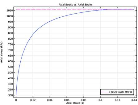
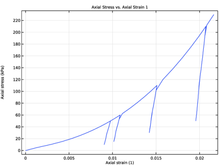
In the Settings window for 1D Plot Group, type Axial Stress vs. Axial Strain in the Label text field.
3
Click to expand the Title section. From the Title type list, choose Label.
4
Locate the Plot Settings section.
5
Select the x-axis label checkbox. In the associated text field, type Axial strain (1).
6
Select the y-axis label checkbox. In the associated text field, type Axial stress (kPa).
7
Locate the Legend section. From the Position list, choose Lower right.
Point Graph 1
1
Right-click Axial Stress vs. Axial Strain and choose Point Graph.
2
3
In the Settings window for Point Graph, locate the y-Axis Data section.
4
In the Expression text field, type -solid.SZZ.
5
Locate the x-Axis Data section. From the Parameter list, choose Expression.
6
In the Expression text field, type -solid.eZZ.
Point Graph 2
1
Right-click Point Graph 1 and choose Duplicate.
2
In the Settings window for Point Graph, locate the y-Axis Data section.
3
In the Expression text field, type -sigmafc.
4
Click to expand the Coloring and Style section. Find the Line style subsection. From the Line list, choose Dashed.
5
From the Color list, choose Magenta.
6
Click to expand the Legends section. Select the Show legends checkbox.
7
From the Legends list, choose Manual.
8
9
In the Axial Stress vs. Axial Strain toolbar, click  Plot.
von Mises Stress vs. Axial Strain
1
In the Results toolbar, click  1D Plot Group.
2
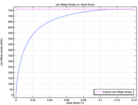
In the Settings window for 1D Plot Group, type von Mises Stress vs. Axial Strain in the Label text field.
3
Locate the Title section. From the Title type list, choose Label.
4
Locate the Plot Settings section.
5
Select the x-axis label checkbox. In the associated text field, type Axial strain (1).
6
Select the y-axis label checkbox. In the associated text field, type von Mises stress (kPa).
7
Locate the Legend section. From the Position list, choose Lower right.
Point Graph 1
1
Right-click von Mises Stress vs. Axial Strain and choose Point Graph.
2
3
In the Settings window for Point Graph, locate the y-Axis Data section.
4
In the Expression text field, type solid.mises.
5
Locate the x-Axis Data section. From the Parameter list, choose Expression.
6
In the Expression text field, type -solid.eZZ.
Point Graph 2
1
Right-click Point Graph 1 and choose Duplicate.
2
In the Settings window for Point Graph, locate the y-Axis Data section.
3
In the Expression text field, type -sigmafc-p0.
4
Locate the Coloring and Style section. Find the Line style subsection. From the Line list, choose Dashed.
5
From the Color list, choose Magenta.
6
Locate the Legends section. Select the Show legends checkbox.
7
From the Legends list, choose Manual.
8
9
In the von Mises Stress vs. Axial Strain toolbar, click  Plot.
Volumetric Strain vs. Axial Strain
1
In the Results toolbar, click  1D Plot Group.
2
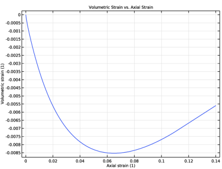
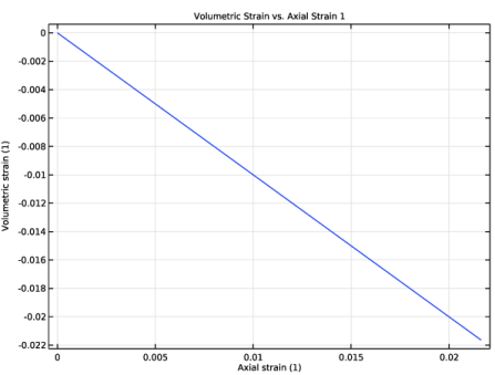
In the Settings window for 1D Plot Group, type Volumetric Strain vs. Axial Strain in the Label text field.
3
Locate the Title section. From the Title type list, choose Label.
4
Locate the Plot Settings section.
5
Select the x-axis label checkbox. In the associated text field, type Axial strain (1).
6
Select the y-axis label checkbox. In the associated text field, type Volumetric strain (1).
Point Graph 1
1
Right-click Volumetric Strain vs. Axial Strain and choose Point Graph.
2
3
In the Settings window for Point Graph, locate the y-Axis Data section.
4
In the Expression text field, type solid.evol.
5
Locate the x-Axis Data section. From the Parameter list, choose Expression.
6
In the Expression text field, type -solid.eZZ.
7
In the Volumetric Strain vs. Axial Strain toolbar, click  Plot.
Mobilized Dilatancy Angle vs. Mobilized Friction Angle
1
In the Results toolbar, click  1D Plot Group.
2
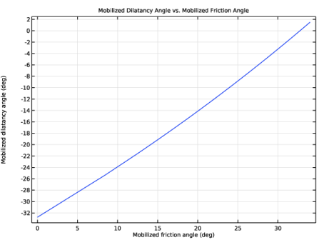
In the Settings window for 1D Plot Group, type Mobilized Dilatancy Angle vs. Mobilized Friction Angle in the Label text field.
3
Locate the Title section. From the Title type list, choose Label.
4
Locate the Plot Settings section.
5
Select the x-axis label checkbox. In the associated text field, type Mobilized friction angle (deg).
6
Select the y-axis label checkbox. In the associated text field, type Mobilized dilatancy angle (deg).
7
Locate the Legend section. From the Position list, choose Upper left.
Point Graph 1
1
Right-click Mobilized Dilatancy Angle vs. Mobilized Friction Angle and choose Point Graph.
2
3
In the Settings window for Point Graph, click Replace Expression in the upper-right corner of the y-Axis Data section. From the menu, choose Component 1 (comp1) > Solid Mechanics > Soil material properties > Hardening soil > solid.epm1.psim - Mobilized dilatancy angle - rad.
4
Locate the y-Axis Data section. In the Expression text field, type solid.epm1.psim*180/pi.
5
Click Replace Expression in the upper-right corner of the x-Axis Data section. From the menu, choose Component 1 (comp1) > Solid Mechanics > Soil material properties > Hardening soil > solid.epm1.phim - Mobilized friction angle - rad.
6
Locate the x-Axis Data section. In the Expression text field, type solid.epm1.phim*180/pi.
7
In the Mobilized Dilatancy Angle vs. Mobilized Friction Angle toolbar, click  Plot.
Axial Stress vs. Axial Strain 1
In the Model Builder window, right-click Axial Stress vs. Axial Strain and choose Duplicate.
Point Graph 2
1
In the Model Builder window, expand the Axial Stress vs. Axial Strain 1 node.
2
Right-click Point Graph 2 and choose Delete.
Axial Stress vs. Axial Strain 1
1
In the Model Builder window, under Results click Axial Stress vs. Axial Strain 1.
2
In the Settings window for 1D Plot Group, locate the Data section.
3
From the Dataset list, choose Study: Oedometer Test/Solution 2 (sol2).
4
In the Axial Stress vs. Axial Strain 1 toolbar, click  Plot.
Volumetric Strain vs. Axial Strain 1
1
In the Model Builder window, right-click Volumetric Strain vs. Axial Strain and choose Duplicate.
2
In the Settings window for 1D Plot Group, locate the Data section.
3
From the Dataset list, choose Study: Oedometer Test/Solution 2 (sol2).
4
In the Volumetric Strain vs. Axial Strain 1 toolbar, click  Plot.
Axial Stress vs. Axial Strain, Mobilized Dilatancy Angle vs. Mobilized Friction Angle, Volumetric Strain vs. Axial Strain, von Mises Stress vs. Axial Strain
1
In the Model Builder window, under Results, Ctrl-click to select Axial Stress vs. Axial Strain, von Mises Stress vs. Axial Strain, Volumetric Strain vs. Axial Strain, and Mobilized Dilatancy Angle vs. Mobilized Friction Angle.
2
Triaxial Test
In the Settings window for Group, type Triaxial Test in the Label text field.
Axial Stress vs. Axial Strain 1, Volumetric Strain vs. Axial Strain 1
1
In the Model Builder window, under Results, Ctrl-click to select Axial Stress vs. Axial Strain 1 and Volumetric Strain vs. Axial Strain 1.
2
Oedometer Test
In the Settings window for Group, type Oedometer Test in the Label text field.