|
|
|
|
•
|
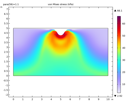
The gravity load is applied using a Gravity node. The pore pressure in the saturated region of the soil sample is applied using an External Stress node.
|
|
•
|
|
1
|
|
2
|
In the Select Physics tree, select Fluid Flow > Porous Media and Subsurface Flow > Richards’ Equation (dl).
|
|
3
|
Right-click and choose Add Physics.
|
|
4
|
|
5
|
Right-click and choose Add Physics.
|
|
6
|
Click
|
|
7
|
|
8
|
Click
|
|
1
|
|
2
|
|
3
|
Click
|
|
4
|
Browse to the model’s Application Libraries folder and double-click the file settlement_analysis_parameters.txt.
|
|
1
|
|
2
|
|
3
|
|
5
|
|
6
|
In the Function table, enter the following settings:
|
|
1
|
|
2
|
|
3
|
|
5
|
|
6
|
In the Function table, enter the following settings:
|
|
1
|
|
2
|
|
3
|
|
4
|
|
5
|
|
6
|
Locate the Units section. In the table, enter the following settings:
|
|
7
|
|
8
|
Locate the Plot Parameters section. In the table, enter the following settings:
|
|
1
|
|
2
|
|
3
|
|
4
|
Click
|
|
5
|
Browse to the model’s Application Libraries folder and double-click the file settlement_analysis_variables.txt.
|
|
1
|
|
2
|
|
3
|
|
4
|
|
1
|
|
2
|
|
3
|
|
4
|
|
5
|
|
6
|
|
7
|
|
8
|
|
9
|
Click
|
|
1
|
|
2
|
|
3
|
|
1
|
|
2
|
|
1
|
In the Model Builder window, under Component 1 (comp1) > Richards’ Equation (dl) click Unsaturated Porous Medium 1.
|
|
2
|
|
3
|
|
1
|
|
2
|
|
3
|
|
4
|
|
5
|
|
6
|
|
7
|
|
1
|
|
3
|
|
4
|
|
1
|
|
1
|
|
2
|
|
3
|
|
1
|
|
2
|
In the Settings window for Elastoplastic Soil Material, type Modified Cam-Clay Model (MCC) in the Label text field.
|
|
4
|
|
5
|
|
6
|
|
7
|
|
1
|
|
2
|
|
3
|
|
4
|
|
5
|
|
6
|
|
1
|
|
2
|
|
1
|
|
2
|
In the Settings window for Elastoplastic Soil Material, type Extended Barcelona Basic Model (BBMx) in the Label text field.
|
|
3
|
Locate the Elastoplastic Soil Material section. From the Material model list, choose Extended Barcelona basic.
|
|
5
|
|
6
|
|
7
|
|
8
|
|
9
|
|
10
|
|
1
|
|
2
|
|
3
|
|
4
|
|
5
|
|
6
|
|
1
|
|
2
|
|
4
|
|
1
|
|
2
|
|
1
|
|
1
|
|
1
|
|
1
|
|
3
|
|
4
|
|
1
|
|
2
|
|
3
|
|
1
|
|
2
|
|
1
|
|
2
|
|
3
|
|
4
|
|
5
|
Locate the Physics and Variables Selection section. Select the Modify model configuration for study step checkbox.
|
|
6
|
In the tree, select Component 1 (comp1) > Solid Mechanics (solid) > Extended Barcelona Basic Model (BBMx).
|
|
7
|
Right-click and choose Disable.
|
|
8
|
|
9
|
Click
|
|
11
|
|
1
|
|
2
|
Go to the Result Templates window.
|
|
3
|
In the tree, select Study: MCC/Solution 1 (sol1) > Solid Mechanics > Volumetric Plastic Strain (solid), Study: MCC/Solution 1 (sol1) > Solid Mechanics > Void Ratio (solid), and Study: MCC/Solution 1 (sol1) > Solid Mechanics > Applied Loads (solid).
|
|
4
|
Click the Add Result Template button in the window toolbar.
|
|
5
|
|
1
|
|
2
|
Go to the Add Study window.
|
|
3
|
|
4
|
Right-click and choose Add Study.
|
|
5
|
|
1
|
|
2
|
|
1
|
|
2
|
|
3
|
|
4
|
|
5
|
|
6
|
Click
|
|
1
|
|
2
|
|
3
|
In the Model Builder window, expand the Study: BBMx > Solver Configurations > Solution 2 (sol2) > Stationary Solver 1 node, then click Parametric 1.
|
|
4
|
|
5
|
Select the Tuning of step size checkbox.
|
|
6
|
|
7
|
|
1
|
|
2
|
|
3
|
|
4
|
|
5
|
Click to expand the Advanced section. Find the Space variables subsection. Select the Remove elements on the symmetry axis checkbox.
|
|
1
|
|
2
|
|
3
|
|
1
|
|
2
|
|
3
|
Click
|
|
4
|
|
5
|
Click OK.
|
|
6
|
|
8
|
Select the Apply conversions to expressions with the same dimensions checkbox.
|
|
9
|
Click
|
|
1
|
|
2
|
|
3
|
|
4
|
|
1
|
|
2
|
|
3
|
|
4
|
|
1
|
|
2
|
|
3
|
|
4
|
|
1
|
|
2
|
|
3
|
|
5
|
|
1
|
|
2
|
|
3
|
|
4
|
|
5
|
|
6
|
|
7
|
|
8
|
|
1
|
|
2
|
In the Settings window for 2D Plot Group, type Degree of Saturation at GWL = 3[m] in the Label text field.
|
|
3
|
|
4
|
|
5
|
|
1
|
In the Model Builder window, under Results > Degree of Saturation at GWL = 3[m], Ctrl-click to select Contour 1 and Streamline 1.
|
|
2
|
Right-click and choose Delete.
|
|
1
|
|
2
|
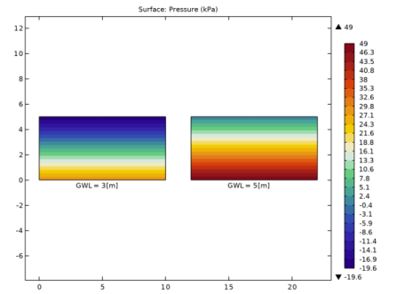
In the Settings window for Surface, click Replace Expression in the upper-right corner of the Expression section. From the menu, choose Component 1 (comp1) > Richards’ Equation > Retention model > dl.Se - Effective saturation - 1.
|
|
1
|
|
2
|
|
1
|
|
2
|
|
3
|
|
4
|
|
1
|
|
2
|
|
3
|
|
4
|
|
1
|
|
2
|
|
3
|
|
4
|
|
5
|
|
1
|
|
2
|
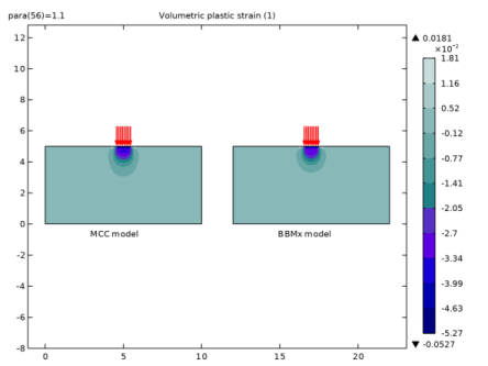
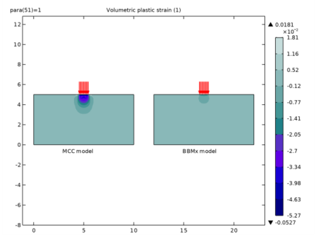
In the Settings window for 2D Plot Group, type Volumetric Plastic Strain at GWL = 3[m] in the Label text field.
|
|
3
|
|
4
|
|
5
|
|
1
|
In the Model Builder window, expand the Volumetric Plastic Strain at GWL = 3[m] node, then click Surface 1.
|
|
2
|
|
3
|
|
1
|
|
2
|
|
3
|
|
4
|
|
5
|
|
6
|
|
1
|
|
2
|
|
3
|
|
1
|
In the Volumetric Plastic Strain at GWL = 3[m] toolbar, click
|
|
2
|
|
3
|
|
5
|
|
1
|
|
2
|
In the Settings window for Arrow Line, click Replace Expression in the upper-right corner of the Expression section. From the menu, choose Component 1 (comp1) > Solid Mechanics > Load > solid.fax,solid.fay - Force per deformed area (spatial frame).
|
|
3
|
|
4
|
|
1
|
|
2
|
|
3
|
|
1
|
|
2
|
|
1
|
|
2
|
Drag and drop Volumetric Plastic Strain at GWL = 3[m] 1 below Volumetric Plastic Strain at GWL = 3[m].
|
|
3
|
In the Settings window for 2D Plot Group, type Volumetric Plastic Strain at GWL = 5[m] in the Label text field.
|
|
4
|
|
1
|
In the Model Builder window, expand the Volumetric Plastic Strain at GWL = 5[m] node, then click Surface 2.
|
|
2
|
|
3
|
|
1
|
|
2
|
|
1
|
|
2
|
|
3
|
|
4
|
|
5
|
|
1
|
|
2
|
|
3
|
|
4
|
|
5
|
|
6
|
|
7
|
|
1
|
|
2
|
|
3
|
|
1
|
|
2
|
|
3
|
|
4
|
Click
|
|
1
|
|
2
|
|
1
|
|
2
|
Drag and drop below Void Ratio at GWL = 5[m].
|
|
3
|
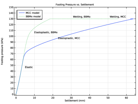
In the Settings window for 1D Plot Group, type Footing Pressure vs. Settlement in the Label text field.
|
|
4
|
|
5
|
Locate the Plot Settings section.
|
|
6
|
|
7
|
|
8
|
|
9
|
|
10
|
|
11
|
|
12
|
|
1
|
|
3
|
|
4
|
|
5
|
|
6
|
|
7
|
|
8
|
|
9
|
|
10
|
|
1
|
|
2
|
|
3
|
|
4
|
Locate the x-Axis Data section. In the Expression text field, type abs(v-withsol('sol2',v,setval(para,0))).
|
|
5
|
Locate the Coloring and Style section. Find the Line style subsection. From the Line list, choose Dotted.
|
|
6
|
Locate the Legends section. In the table, enter the following settings:
|
|
1
|
|
2
|
|
3
|
|
5
|
|
1
|
|
2
|
|
1
|
|
2
|
|
3
|
|
4
|
|
5
|
|
6
|
|
1
|
|
2
|
|
3
|
|
1
|
|
2
|
Drag and drop below Footing Pressure vs. Settlement.
|
|
3
|
|
4
|
|
5
|
|
6
|
|
7
|
|
8
|
Locate the Plot Settings section.
|
|
9
|
|
10
|
|
11
|
|
1
|
|
2
|
|
3
|
|
4
|
|
5
|
|
6
|
|
7
|
|
8
|
|
1
|
|
2
|
|
3
|
|
4
|
|
5
|
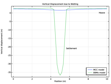
Locate the y-Axis Data section. In the Expression text field, type v-withsol('sol2',v,setval(para,1)).
|
|
6
|
Locate the Legends section. In the table, enter the following settings:
|
|
1
|
|
2
|
|
3
|
|
5
|
|
1
|
|
2
|