|
|
|
|
•
|
The four clays analyzed here are naturally structured Osaka clay, naturally structured Marl clay, artificially structured Ariake clay, and artificially structured Bangkok clay. Also, different cement contents by weight (Aw) are considered for the two artificially structured clays.
|
|
•
|
The common material parameters are density ρ = 2000 kg/m3, reference pressure pref = 1 kPa, and critical effective deviatoric plastic strain εdcp = 0.1.
|
|
•
|
Material properties like the shear modulus G, slope of critical state line M, compression index for destructured clay λd, swelling index for structured clay κs, void ratio at reference pressure for destructured clay erefd, additional void ratio at initial yielding Δei, plastic potential shape parameter ζ, destructuring index for volumetric deformation dv, destructuring index for shear deformation ds, initial consolidation pressure pc0, and initial structure strength pbi for the four different clays are shown in Table 1, Table 2, and Table 3.
|
|
1
|
|
2
|
|
3
|
Click Add.
|
|
4
|
Click
|
|
5
|
|
6
|
Click
|
|
1
|
|
2
|
|
3
|
|
4
|
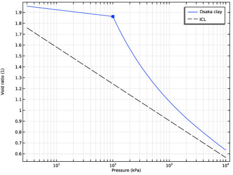
Browse to the model’s Application Libraries folder and double-click the file isotropic_compression_mscc_osaka_parameters.txt.
|
|
5
|
|
6
|
|
7
|
|
8
|
|
9
|
Click
|
|
10
|
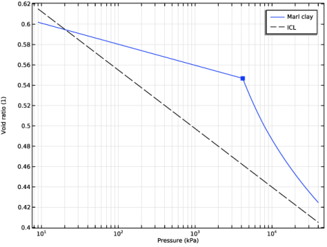
Browse to the model’s Application Libraries folder and double-click the file isotropic_compression_mscc_marl_parameters.txt.
|
|
11
|
|
12
|
|
13
|
|
14
|
Click
|
|
15
|
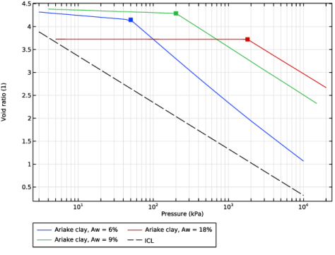
Browse to the model’s Application Libraries folder and double-click the file isotropic_compression_mscc_ariake_Aw6_parameters.txt.
|
|
16
|
|
17
|
|
18
|
|
19
|
Click
|
|
20
|
Browse to the model’s Application Libraries folder and double-click the file isotropic_compression_mscc_ariake_Aw9_parameters.txt.
|
|
21
|
|
22
|
|
23
|
|
24
|
Click
|
|
25
|
Browse to the model’s Application Libraries folder and double-click the file isotropic_compression_mscc_ariake_Aw18_parameters.txt.
|
|
26
|
|
27
|
|
28
|
|
29
|
Click
|
|
30
|
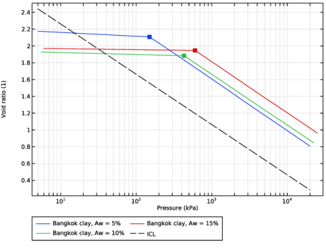
Browse to the model’s Application Libraries folder and double-click the file isotropic_compression_mscc_bangkok_Aw5_parameters.txt.
|
|
31
|
|
32
|
|
33
|
|
34
|
Click
|
|
35
|
Browse to the model’s Application Libraries folder and double-click the file isotropic_compression_mscc_bangkok_Aw10_parameters.txt.
|
|
36
|
|
37
|
|
38
|
|
39
|
Click
|
|
40
|
Browse to the model’s Application Libraries folder and double-click the file isotropic_compression_mscc_bangkok_Aw15_parameters.txt.
|
|
41
|
|
1
|
|
2
|
|
1
|
|
2
|
|
3
|
|
1
|
|
2
|
|
3
|
|
4
|
|
5
|
Click
|
|
1
|
In the Model Builder window, under Component 1 (comp1) right-click Materials and choose Blank Material.
|
|
2
|
|
1
|
|
2
|
|
3
|
|
4
|
Locate the Elastoplastic Soil Material section. From the Material model list, choose Modified structured Cam-clay.
|
|
5
|
|
6
|
|
7
|
|
8
|
|
9
|
|
10
|
|
11
|
|
12
|
In the Show More Options dialog, in the tree, select the checkbox for the node Physics > Advanced Physics Options.
|
|
13
|
Click OK.
|
|
14
|
|
15
|
|
16
|
|
17
|
|
1
|
|
3
|
|
4
|
|
5
|
|
1
|
|
1
|
|
2
|
|
1
|
|
2
|
|
3
|
|
4
|
|
5
|
Click
|
|
1
|
|
2
|
|
3
|
Clear the Generate default plots checkbox.
|
|
1
|
|
2
|
|
3
|
|
4
|
Click
|
|
1
|
|
2
|
|
3
|
Select the Auxiliary sweep checkbox.
|
|
4
|
Click
|
|
6
|
|
1
|
|
2
|
|
3
|
|
4
|
|
5
|
|
6
|
|
7
|
|
8
|
Locate the Plot Settings section.
|
|
9
|
|
10
|
|
1
|
|
3
|
In the Settings window for Point Graph, click Replace Expression in the upper-right corner of the y-Axis Data section. From the menu, choose Component 1 (comp1) > Solid Mechanics > Soil material properties > Modified structured Cam-clay > solid.epm1.evoid - Void ratio - 1.
|
|
4
|
Click Replace Expression in the upper-right corner of the x-Axis Data section. From the menu, choose Component 1 (comp1) > Solid Mechanics > Stress > solid.pmGp - Pressure - N/m².
|
|
5
|
|
6
|
|
7
|
|
1
|
|
2
|
|
3
|
|
4
|
|
5
|
|
6
|
|
7
|
|
8
|
|
1
|
In the Model Builder window, under Results > Natural Osaka Clay right-click Point Graph 1 and choose Duplicate.
|
|
2
|
|
3
|
In the Expression text field, type solid.epm1.evoidrefd-solid.epm1.lambdaCompd*log(solid.epm1.pm/solid.epm1.pref).
|
|
4
|
Locate the Coloring and Style section. Find the Line style subsection. From the Line list, choose Dashed.
|
|
5
|
|
6
|
Locate the Legends section. In the table, enter the following settings:
|
|
7
|
|
1
|
|
2
|
|
3
|
|
1
|
|
2
|
|
4
|
|
1
|
|
2
|
|
3
|
Locate the Data section. In the Clay Material Properties list, choose Cemented Ariake Clay, Aw = 6%, Cemented Ariake Clay, Aw = 9%, and Cemented Ariake Clay, Aw = 18%.
|
|
1
|
|
2
|
|
1
|
|
2
|
|
3
|
|
4
|
|
5
|
|
1
|
|
2
|
|
3
|
|
4
|
|
5
|
|
6
|
|
1
|
|
2
|
|
3
|
Locate the Data section. In the Clay Material Properties list, choose Cemented Bangkok Clay, Aw = 5%, Cemented Bangkok Clay, Aw = 10%, and Cemented Bangkok Clay, Aw = 15%.
|
|
1
|
|
2
|
|
1
|
|
2
|
|
3
|
|
4
|