PDF

Hysteresis in Soil Using the Small-Strain Overlay Model
Introduction
The majority of soil types have a high stiffness at small strains in the elastic regime while it decreases monotonically with increasing strain. Soils also displays a hysteresis effect when subjected to cyclic loads. The Small-Strain Overlay model presented in Ref. 1 captures the effect of high stiffness at low strain as well as the hysteric behavior under cyclic loading. The formulation allows stiffness degradation with an increase in shear strain, and the full recovery of stiffness at load reversal.
In this example, cyclic tensile and shear tests show the stiffness degradation and the hysteresis effect with the small-strain overlay model. The cyclic tensile test mimic the cyclic triaxial loading without any isotropic compression step.
Model Definition
A rectangular soil specimen of 5 cm in width and 10 cm in height is used for both tests. The specimen is represented by a 2D geometry.
Soil Properties
Properties for dense sand are presented in Table 1 as taken from Ref. 1.
ν
ρ
G0
Constraints and Loads
Results and Discussion
Note that for consistency with the geomechanics sign convention, compressive stress and strain are plotted along the positive axis in all figures, while tensile stress and strain are plotted along the negative axis.
For the cyclic triaxial test, the axial stress versus axial strain is shown in Figure 1, while the variation of Young’s modulus versus axial strain is shown in Figure 2. The small-strain overlay model captures two important aspects of the behavior of soils:
From Figure 1 it is clear that the model satisfies two basic rules of Masing:
Note that a log scale is used for the axial strain in the Figure 2, which is why the first parametric steps corresponding to zero strain are excluded. The stiffness at the beginning of the unloading curve is the same as the initial stiffness at the beginning of the primary loading.
The hysteresis effect in the cyclic shear test is shown in Figure 3. Figure 4 shows a reduction in the shear stiffness with increasing shear strain. From both figures it can be observed that the stiffness at the start of the unloading cycle is regained and that both Massing rules are satisfied.
Figure 1: Axial stress versus axial strain for the cyclic tensile test.
Figure 2: Young’s modulus versus axial strain for the cyclic tensile test.
.
Figure 3: Shear stress versus shear strain in the cyclic shear test.
Figure 4: Shear modulus versus shear strain in the cyclic shear test.
Notes About the COMSOL Implementation
For cyclic loading, the load reversal points in the small-strain overlay model are found automatically based on the increments of the deviatoric strain tensor. However, in some load cases, the automatic algorithm is not effective. In such scenarios the user can set Load reversal points to User defined. With this option, a set of load reversal points can be specified in terms of the parameter for a parametric study or the time variable for a transient study.
Reference
1. T. Benz, P. A. Vermeer, and R. Schwab, “A small-strain overlay model,” Int. J. Numer. Anal. Methods Geomech., vol. 33, pp. 25–44, 2009.
Application Library path: Geomechanics_Module/Verification_Examples/hysteresis_small_strain_overlay
Modeling Instructions
From the File menu, choose New.
New
In the New window, click  Model Wizard.
Model Wizard
1
In the Model Wizard window, click  2D.
2
In the Select Physics tree, select Structural Mechanics > Solid Mechanics (solid).
3
Click Add.
4
Click  Study.
5
In the Select Study tree, select General Studies > Stationary.
6
Global Definitions
Parameters 1
1
In the Model Builder window, under Global Definitions click Parameters 1.
2
In the Settings window for Parameters, locate the Parameters section.
3
Definitions
Interpolation 1 (int1)
1
In the Definitions toolbar, click  Interpolation.
2
In the Settings window for Interpolation, locate the Definition section.
3
In the Function name text field, type appliedDisp.
4
5
Locate the Units section. In the Function table, enter the following settings:
6
In the Argument table, enter the following settings:
Geometry 1
Rectangle 1 (r1)
1
In the Geometry toolbar, click  Rectangle.
2
In the Settings window for Rectangle, locate the Size and Shape section.
3
In the Width text field, type 5[cm].
4
In the Height text field, type 10[cm].
5
Click  Build Selected.
Solid Mechanics (solid)
1
In the Model Builder window, under Component 1 (comp1) click Solid Mechanics (solid).
2
In the Settings window for Solid Mechanics, click to expand the Discretization section.
3
From the Displacement field list, choose Linear.
Nonlinear Elastic Material 1
1
In the Physics toolbar, click  Domains and choose Nonlinear Elastic Material.
2
3
In the Settings window for Nonlinear Elastic Material, locate the Nonlinear Elastic Material section.
4
From the Material model list, choose Small-strain overlay.
Roller 1
1
In the Physics toolbar, click  Boundaries and choose Roller.
2
Prescribed Displacement 1
1
In the Physics toolbar, click  Boundaries and choose Prescribed Displacement.
2
3
In the Settings window for Prescribed Displacement, locate the Prescribed Displacement section.
4
From the Displacement in y direction list, choose Prescribed.
5
In the u0y text field, type -appliedDisp(para).
Prescribed Displacement 2
1
In the Physics toolbar, click  Boundaries and choose Prescribed Displacement.
2
3
In the Settings window for Prescribed Displacement, locate the Prescribed Displacement section.
4
From the Displacement in y direction list, choose Prescribed.
5
In the u0y text field, type appliedDisp(para).
Prescribed Displacement 3
1
Right-click Prescribed Displacement 2 and choose Duplicate.
2
In the Settings window for Prescribed Displacement, locate the Boundary Selection section.
3
Click  Clear Selection.
4
5
Locate the Prescribed Displacement section. In the u0y text field, type 0.
Prescribed Displacement 4
1
In the Physics toolbar, click  Boundaries and choose Prescribed Displacement.
2
3
In the Settings window for Prescribed Displacement, locate the Prescribed Displacement section.
4
From the Displacement in x direction list, choose Prescribed.
5
In the u0x text field, type appliedDisp(para).
Prescribed Displacement 5
1
Right-click Prescribed Displacement 4 and choose Duplicate.
2
In the Settings window for Prescribed Displacement, locate the Boundary Selection section.
3
Click  Clear Selection.
4
5
Locate the Prescribed Displacement section. In the u0x text field, type 0.
Prescribed Displacement 1, Roller 1
1
In the Model Builder window, under Component 1 (comp1) > Solid Mechanics (solid), Ctrl-click to select Roller 1 and Prescribed Displacement 1.
2
Cyclic Triaxial Loading
In the Settings window for Group, type Cyclic Triaxial Loading in the Label text field.
Prescribed Displacement 2, Prescribed Displacement 3, Prescribed Displacement 4, Prescribed Displacement 5
1
In the Model Builder window, under Component 1 (comp1) > Solid Mechanics (solid), Ctrl-click to select Prescribed Displacement 2, Prescribed Displacement 3, Prescribed Displacement 4, and Prescribed Displacement 5.
2
Cyclic Shear Loading
In the Settings window for Group, type Cyclic Shear Loading in the Label text field.
Materials
Soil Material
1
In the Model Builder window, under Component 1 (comp1) right-click Materials and choose Blank Material.
2
In the Settings window for Material, type Soil Material in the Label text field.
3
Locate the Material Contents section. In the table, enter the following settings:
One mesh element is sufficient for this analysis.
Mesh 1
Mapped 1
In the Mesh toolbar, click  Mapped.
Distribution 1
1
Right-click Mapped 1 and choose Distribution.
2
In the Settings window for Distribution, locate the Boundary Selection section.
3
From the Selection list, choose All boundaries.
4
Locate the Distribution section. In the Number of elements text field, type 1.
5
Click  Build Selected.
Study: Cyclic Triaxial Loading
Disable the default plots for this study.
1
In the Model Builder window, click Study 1.
2
In the Settings window for Study, type Study: Cyclic Triaxial Loading in the Label text field.
3
Locate the Study Settings section. Clear the Generate default plots checkbox.
Step 1: Stationary
1
In the Model Builder window, under Study: Cyclic Triaxial Loading click Step 1: Stationary.
2
In the Settings window for Stationary, locate the Physics and Variables Selection section.
3
Select the Modify model configuration for study step checkbox.
4
In the tree, select Component 1 (comp1) > Solid Mechanics (solid) > Cyclic Shear Loading.
5
6
Click to expand the Study Extensions section. Select the Auxiliary sweep checkbox.
7
8
9
In the Study toolbar, click  Compute.
Add a second study for the cyclic shear loading.
Add Study
1
In the Home toolbar, click  Add Study to open the Add Study window.
2
Go to the Add Study window.
3
Find the Studies subsection. In the Select Study tree, select General Studies > Stationary.
4
Click the Add Study button in the window toolbar.
5
In the Home toolbar, click  Add Study to close the Add Study window.
Study: Cyclic Shear Loading
Disable the default plots for this study.
1
In the Settings window for Study, type Study: Cyclic Shear Loading in the Label text field.
2
Locate the Study Settings section. Clear the Generate default plots checkbox.
1
In the Model Builder window, under Study: Cyclic Shear Loading click Step 1: Stationary.
2
In the Settings window for Stationary, locate the Study Extensions section.
3
Select the Auxiliary sweep checkbox.
4
5
6
In the Study toolbar, click  Compute.
Results
Axial Stress vs. Axial Strain
1
In the Results toolbar, click  1D Plot Group.
2
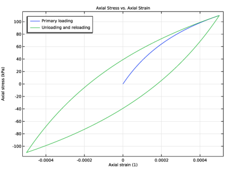
In the Settings window for 1D Plot Group, type Axial Stress vs. Axial Strain in the Label text field.
3
Click to expand the Title section. From the Title type list, choose Manual.
4
In the Title text area, type Axial Stress vs. Axial Strain.
5
Locate the Plot Settings section.
6
Select the x-axis label checkbox. In the associated text field, type Axial strain (1).
7
Select the y-axis label checkbox. In the associated text field, type Axial stress (kPa).
8
Locate the Legend section. From the Position list, choose Upper left.
Point Graph 1
1
Right-click Axial Stress vs. Axial Strain and choose Point Graph.
2
In the Settings window for Point Graph, locate the Data section.
3
From the Dataset list, choose Study: Cyclic Triaxial Loading/Solution 1 (sol1).
4
From the Parameter selection (para) list, choose Manual.
5
In the Parameter indices (1-5001) text field, type range(1,1,1001).
6
7
Locate the y-Axis Data section. In the Expression text field, type -solid.SYY.
8
From the Unit list, choose kPa.
9
Locate the x-Axis Data section. From the Parameter list, choose Expression.
10
In the Expression text field, type -solid.eYY.
11
Click to expand the Legends section. Select the Show legends checkbox.
12
From the Legends list, choose Manual.
13
Point Graph 2
1
Right-click Point Graph 1 and choose Duplicate.
2
In the Settings window for Point Graph, locate the Data section.
3
In the Parameter indices (1-5001) text field, type range(1001,1,5001).
4
Locate the Legends section. In the table, enter the following settings:
Axial Stress vs. Axial Strain
1
In the Model Builder window, click Axial Stress vs. Axial Strain.
2
In the Axial Stress vs. Axial Strain toolbar, click  Plot.
Young’s Modulus vs. Axial Strain
1
Right-click Axial Stress vs. Axial Strain and choose Duplicate.
2
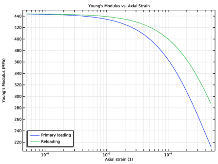
In the Settings window for 1D Plot Group, type Young's Modulus vs. Axial Strain in the Label text field.
3
Locate the Title section. In the Title text area, type Young's Modulus vs. Axial Strain.
4
Locate the Plot Settings section. In the y-axis label text field, type Young's Modulus (MPa).
Point Graph 1
1
In the Model Builder window, expand the Young’s Modulus vs. Axial Strain node, then click Point Graph 1.
2
In the Settings window for Point Graph, locate the y-Axis Data section.
3
In the Expression text field, type solid.E.
4
From the Unit list, choose MPa.
5
Locate the x-Axis Data section. In the Expression text field, type abs(solid.eYY).
Point Graph 2
1
In the Model Builder window, click Point Graph 2.
2
In the Settings window for Point Graph, locate the Data section.
3
In the Parameter indices (1-5001) text field, type range(3002,1,4001).
4
Locate the y-Axis Data section. In the Expression text field, type solid.E.
5
From the Unit list, choose MPa.
6
Locate the x-Axis Data section. In the Expression text field, type abs(solid.eYY-withsol('sol1',solid.eYY,setval(para,3))).
7
Locate the Legends section. In the table, enter the following settings:
Young’s Modulus vs. Axial Strain
1
In the Model Builder window, click Young’s Modulus vs. Axial Strain.
2
In the Settings window for 1D Plot Group, locate the Axis section.
3
Select the x-axis log scale checkbox.
4
Locate the Legend section. From the Position list, choose Lower left.
5
In the Young’s Modulus vs. Axial Strain toolbar, click  Plot.
Shear Stress vs. Shear Strain
1
In the Model Builder window, right-click Axial Stress vs. Axial Strain and choose Duplicate.
2
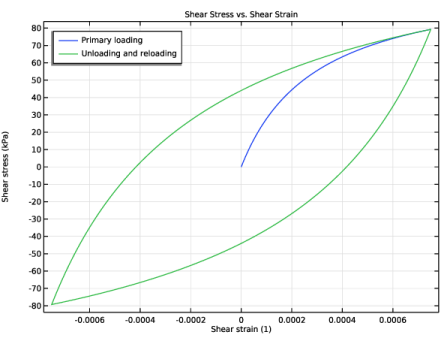
In the Settings window for 1D Plot Group, type Shear Stress vs. Shear Strain in the Label text field.
3
Locate the Data section. From the Dataset list, choose Study: Cyclic Shear Loading/Solution 2 (sol2).
4
Locate the Title section. In the Title text area, type Shear Stress vs. Shear Strain.
5
Locate the Plot Settings section. In the x-axis label text field, type Shear strain (1).
6
In the y-axis label text field, type Shear stress (kPa).
Point Graph 1
1
In the Model Builder window, expand the Shear Stress vs. Shear Strain node, then click Point Graph 1.
2
In the Settings window for Point Graph, locate the Data section.
3
From the Dataset list, choose Study: Cyclic Shear Loading/Solution 2 (sol2).
4
Locate the y-Axis Data section. In the Expression text field, type solid.SXY.
5
Locate the x-Axis Data section. In the Expression text field, type solid.eXY.
Point Graph 2
1
In the Model Builder window, click Point Graph 2.
2
In the Settings window for Point Graph, locate the Data section.
3
From the Dataset list, choose Study: Cyclic Shear Loading/Solution 2 (sol2).
4
Locate the y-Axis Data section. In the Expression text field, type solid.SXY.
5
Locate the x-Axis Data section. In the Expression text field, type solid.eXY.
6
In the Shear Stress vs. Shear Strain toolbar, click  Plot.
Shear Modulus vs. Shear Strain
1
In the Model Builder window, right-click Young’s Modulus vs. Axial Strain and choose Duplicate.
2
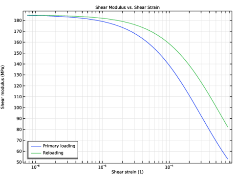
In the Settings window for 1D Plot Group, type Shear Modulus vs. Shear Strain in the Label text field.
3
Locate the Data section. From the Dataset list, choose Study: Cyclic Shear Loading/Solution 2 (sol2).
4
Locate the Title section. In the Title text area, type Shear Modulus vs. Shear Strain.
5
Locate the Plot Settings section. In the x-axis label text field, type Shear strain (1).
6
In the y-axis label text field, type Shear modulus (MPa).
Point Graph 1
1
In the Model Builder window, expand the Shear Modulus vs. Shear Strain node, then click Point Graph 1.
2
In the Settings window for Point Graph, locate the Data section.
3
From the Dataset list, choose Study: Cyclic Shear Loading/Solution 2 (sol2).
4
Locate the y-Axis Data section. In the Expression text field, type solid.G.
5
Locate the x-Axis Data section. In the Expression text field, type abs(solid.eXY).
Point Graph 2
1
In the Model Builder window, click Point Graph 2.
2
In the Settings window for Point Graph, locate the Data section.
3
From the Dataset list, choose Study: Cyclic Shear Loading/Solution 2 (sol2).
4
Locate the y-Axis Data section. In the Expression text field, type solid.G.
5
Locate the x-Axis Data section. In the Expression text field, type abs(solid.eXY-withsol('sol2',solid.eXY,setval(para,3))).
6
In the Shear Modulus vs. Shear Strain toolbar, click  Plot.
Axial Stress vs. Axial Strain, Young’s Modulus vs. Axial Strain
1
In the Model Builder window, under Results, Ctrl-click to select Axial Stress vs. Axial Strain and Young’s Modulus vs. Axial Strain.
2
Triaxial Loading
In the Settings window for Group, type Triaxial Loading in the Label text field.
Shear Modulus vs. Shear Strain, Shear Stress vs. Shear Strain
1
In the Model Builder window, under Results, Ctrl-click to select Shear Stress vs. Shear Strain and Shear Modulus vs. Shear Strain.
2
Shear Loading
In the Settings window for Group, type Shear Loading in the Label text field.