PDF

Flexible and Smooth Strip Footing on a Stratum of Clay
Model Definition
A typical verification example for geotechnical problems is a shallow stratum layer of clay, see Figure 1. In the example, a vertical load is applied on the clay stratum, and the static response as well as the collapse load are of interest. This example is adapted from Ref. 2.
Figure 1: Dimensions, boundary conditions, and pressure load for the stratum of clay.
Analysis Type
Yield Surface
Assume plane strain conditions, and model the clay with soil plasticity and the Drucker–Prager criterion.
The yield surface, F, for the Drucker–Prager criterion is given by
where I1 is the first stress invariant and J2 is the second deviatoric stress invariant.
The first stress invariant is defined as the trace of Cauchy stress tensor:
The second stress invariant is defined as
The second deviatoric stress invariant can be expressed using the first and the second stress invariants:
If 2D plane strain conditions prevail, the Drucker–Prager criterion matches the Mohr–Coulomb criterion. For this case the material parameters α and k are given by the cohesion c and the angle of internal friction ϕ (Ref. 1)
The Drucker–Prager criterion is the default choice for the Soil Plasticity feature, and the checkbox Match to Mohr–Coulomb criterion applies the aforementioned matching of the material parameters.
Under Soil Plasticity, it is also possible to use Mohr–Coulomb criterion
,
where σmax and σmin are the biggest and smallest principal stresses, respectively. The Mohr–Coulomb criterion defines an irregular hexagon pyramid in the principal stress space. Since this yield function gives rise to singularities in the derivatives of the yield function, the use of a nonassociated flow rule with a Drucker–Prager plastic potential is chosen. This is done in the plastic potential list, with the option Drucker–Prager matched at compressive meridian.
Flow Rule
The flow rule defines the relation between the plastic strain increment in a given direction and the current level of stress in the same direction. The relation reads
where λ is the plastic multiplier and Q is the plastic potential. If the yield surface, F, and the plastic potential, Q, are identical, that is, if = Q, then it is called an associated flow rule, otherwise it is called a nonassociated flow rule.
Soil Properties
Young’s modulus, E = 207 MPa, and Poisson’s ratio ν = 0.3.
Cohesion c = 69 kPa, and angle of internal friction  = 20°.
Constraints and Loads
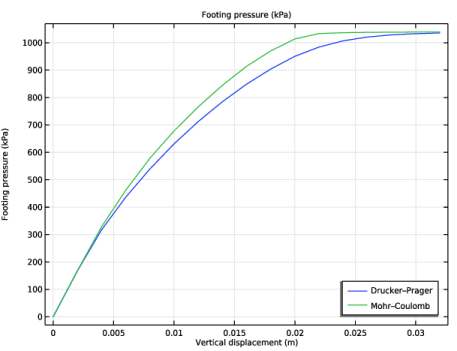
The stratum is subjected to a footing that is considered to be flexible and smooth. The width of the strip footing is 3.14 m, see Figure 2. Gradually increase the footing pressure until the clay layer reaches the collapse load.
Infinite Element Domain
In order to mimic an infinite layer of soil, add an Infinite Element Domain. The scaling 1e3*root.mod1.dGeomChar means that the spatial variables in this domain are scaled by thousand times the typical geometry length.
Results and Discussion
The load-displacement curves for both the Mohr–Coulomb and the Drucker–Prager criteria are plotted in Figure 2. The relation between the applied footing pressure and the centerline displacement (directly beneath the center of the footing) in the y direction are shown. The lines show the load-displacement curves for the Mohr–Coulomb and Drucker–Prager criteria. The curves are identical up to 300 kPa because the whole domain is still within the elastic region. From that point when the pressure increases, the behavior diverges. Both curves reach the collapse load at approximately 1.1 MPa. The development of plastic strains in the soil at different stages of loading is shown in Figure 3.
Figure 2: Footing pressure versus vertical displacement for the Mohr–Coulomb and Drucker–Prager material models.
Figure 3: Evolution of the equivalent plastic strain on the clay layer during the parametric loading. Dark regions indicate the plastic region.
Notes About the COMSOL Implementation
A suitable modeling technique in a case where the relation between the applied load and the displacement is highly nonlinear, is to use an algebraic equation that controls the applied pressure so that the model reaches the desired displacement increments. This is implemented using a Global Equation, and the parametric solver incrementally increases the displacement up to the desired vertical displacement.
References
1. W.F. Chen and E. Mizuno, Nonlinear Analysis in Soil Mechanics, Elsevier, 1990.
2. A. Mar, How To Undertake Finite Element Based Geotechnical Analysis, NAFEMS, 2002.
Application Library path: Geomechanics_Module/Soil/flexible_footing
Modeling Instructions
From the File menu, choose New.
New
In the New window, click  Model Wizard.
Model Wizard
1
In the Model Wizard window, click  2D.
2
In the Select Physics tree, select Structural Mechanics > Solid Mechanics (solid).
3
Click Add.
4
Click  Study.
5
In the Select Study tree, select General Studies > Stationary.
6
Global Definitions
Parameters 1
1
In the Model Builder window, under Global Definitions click Parameters 1.
2
In the Settings window for Parameters, locate the Parameters section.
3
Geometry 1
Rectangle 1 (r1)
1
In the Geometry toolbar, click  Rectangle.
2
In the Settings window for Rectangle, locate the Size and Shape section.
3
In the Width text field, type W*1.1.
4
In the Height text field, type H.
5
Locate the Position section. In the x text field, type -W*0.1.
6
Click to expand the Layers section. In the table, enter the following settings:
7
Clear the Layers on bottom checkbox.
8
Select the Layers to the left checkbox.
The left layer is used to model an infinite element domain.
Point 1 (pt1)
1
In the Geometry toolbar, click  Point.
2
In the Settings window for Point, locate the Point section.
3
In the x text field, type W-1.57[m].
4
In the y text field, type H.
Form Union (fin)
1
In the Model Builder window, click Form Union (fin).
2
In the Settings window for Form Union/Assembly, click  Build Selected.
Definitions
Infinite Element Domain 1 (ie1)
1
In the Definitions toolbar, click  Infinite Element Domain.
The infinite element domain is scaled by a factor of 1000.
2
Add a nonlocal integration coupling to evaluate the displacement at the center of the applied pressure (point 7).
Integration 1 (intop1)
1
In the Definitions toolbar, click  Nonlocal Couplings and choose Integration.
2
In the Settings window for Integration, locate the Source Selection section.
3
From the Geometric entity level list, choose Point.
4
Solid Mechanics (solid)
Linear Elastic Material 1
In the Model Builder window, under Component 1 (comp1) > Solid Mechanics (solid) click Linear Elastic Material 1.
Soil Plasticity 1
1
In the Physics toolbar, click  Attributes and choose Soil Plasticity.
2
In the Settings window for Soil Plasticity, locate the Soil Plasticity Model section.
3
From the Match to Mohr–Coulomb list, choose Inscribe (plane strain).
Linear Elastic Material 1
In the Model Builder window, click Linear Elastic Material 1.
Soil Plasticity 2
1
In the Physics toolbar, click  Attributes and choose Soil Plasticity.
2
In the Settings window for Soil Plasticity, locate the Soil Plasticity Model section.
3
From the Ff list, choose Mohr–Coulomb.
Fixed Constraint 1
1
In the Physics toolbar, click  Boundaries and choose Fixed Constraint.
2
Symmetry 1
1
In the Physics toolbar, click  Boundaries and choose Symmetry.
2
Roller 1
1
In the Physics toolbar, click  Boundaries and choose Roller.
2
Boundary Load 1
1
In the Physics toolbar, click  Boundaries and choose Boundary Load.
2
3
In the Settings window for Boundary Load, locate the Force section.
4
Specify the fA vector as
5
Click the  Show More Options button in the Model Builder toolbar.
6
In the Show More Options dialog, in the tree, select the checkbox for the node Physics > Equation Contributions.
7
Global Equations 1 (ODE1)
1
In the Physics toolbar, click  Global and choose Global Equations.
2
In the Settings window for Global Equations, locate the Global Equations section.
3
4
Locate the Units section. Click  Select Dependent Variable Quantity.
5
In the Physical Quantity dialog, type pressure in the text field.
6
In the tree, select General > Pressure (Pa).
7
8
In the Settings window for Global Equations, locate the Units section.
9
Click  Select Source Term Quantity.
10
In the Physical Quantity dialog, type displacement in the text field.
11
In the tree, select General > Displacement (m).
12
Materials
Material 1 (mat1)
1
In the Model Builder window, under Component 1 (comp1) right-click Materials and choose Blank Material.
2
In the Settings window for Material, locate the Material Contents section.
3
Mesh 1
1
In the Model Builder window, under Component 1 (comp1) click Mesh 1.
2
In the Settings window for Mesh, locate the Sequence Type section.
3
From the list, choose User-controlled mesh.
Size
1
In the Model Builder window, under Component 1 (comp1) > Mesh 1 click Size.
2
In the Settings window for Size, locate the Element Size section.
3
From the Predefined list, choose Finer.
Free Triangular 1
1
In the Model Builder window, click Free Triangular 1.
2
In the Settings window for Free Triangular, locate the Domain Selection section.
3
From the Geometric entity level list, choose Domain.
4
Mapped 1
1
In the Mesh toolbar, click  Mapped.
Use a mapped mesh in the infinite element domain to improve convergence.
2
In the Settings window for Mapped, locate the Domain Selection section.
3
From the Geometric entity level list, choose Domain.
4
5
Click  Build All.
The first study is parametric and solves the model assuming the Drucker–Prager criterion. The stepping parameter v_prescr represents the vertical displacement at the center of the applied pressure (point 7).
Study: Drucker–Prager
1
In the Model Builder window, click Study 1.
2
In the Settings window for Study, type Study: Drucker-Prager in the Label text field.
Step 1: Stationary
1
In the Model Builder window, under Study: Drucker–Prager click Step 1: Stationary.
2
In the Settings window for Stationary, locate the Physics and Variables Selection section.
3
Select the Modify model configuration for study step checkbox.
4
In the tree, select Component 1 (comp1) > Solid Mechanics (solid) > Linear Elastic Material 1 > Soil Plasticity 2.
5
Click  Disable.
6
Click to expand the Study Extensions section. Select the Auxiliary sweep checkbox.
7
8
9
In the Study toolbar, click  Compute.
Add a plot from Result Templates to easily visualize the plastic region.
Result Templates
1
In the Results toolbar, click  Result Templates to open the Result Templates window.
2
Go to the Result Templates window.
3
In the tree, select Study: Drucker–Prager/Solution 1 (sol1) > Solid Mechanics > Equivalent Plastic Strain (solid).
4
Click the Add Result Template button in the window toolbar.
Root
The second study is also parametric and solves the model assuming a Mohr–Coulomb criterion. Again, the stepping parameter v_prescr represents the vertical displacement at the center of the applied pressure (point 7).
Add Study
1
In the Home toolbar, click  Add Study to open the Add Study window.
2
Go to the Add Study window.
3
Find the Studies subsection. In the Select Study tree, select General Studies > Stationary.
4
Click the Add Study button in the window toolbar.
5
In the Home toolbar, click  Add Study to close the Add Study window.
Study: Mohr–Coulomb
In the Settings window for Study, type Study: Mohr-Coulomb in the Label text field.
1
In the Model Builder window, under Study: Mohr–Coulomb click Step 1: Stationary.
2
In the Settings window for Stationary, locate the Physics and Variables Selection section.
3
Select the Modify model configuration for study step checkbox.
4
In the tree, select Component 1 (comp1) > Solid Mechanics (solid) > Linear Elastic Material 1 > Soil Plasticity 1.
5
Click  Disable.
6
Locate the Study Extensions section. Select the Auxiliary sweep checkbox.
7
8
9
In the Study toolbar, click  Compute.
Result Templates
1
Go to the Result Templates window.
2
In the tree, select Study: Mohr–Coulomb/Solution 2 (sol2) > Solid Mechanics > Equivalent Plastic Strain (solid).
3
Click the Add Result Template button in the window toolbar.
4
In the Results toolbar, click  Result Templates to close the Result Templates window.
Results
Remove the infinite element domain from the dataset for plotting.
Study: Drucker–Prager/Solution 1 (sol1)
In the Model Builder window, expand the Results > Datasets node, then click Study: Drucker–Prager/Solution 1 (sol1).
Selection
1
In the Results toolbar, click  Attributes and choose Selection.
2
In the Settings window for Selection, locate the Geometric Entity Selection section.
3
From the Geometric entity level list, choose Domain.
4
Study: Mohr–Coulomb/Solution 2 (sol2)
In the Model Builder window, under Results > Datasets click Study: Mohr–Coulomb/Solution 2 (sol2).
Selection
1
In the Results toolbar, click  Attributes and choose Selection.
2
In the Settings window for Selection, locate the Geometric Entity Selection section.
3
From the Geometric entity level list, choose Domain.
4
Add mirror datasets to improve the result visualization.
Mirror 2D 1
1
In the Results toolbar, click  More Datasets and choose Mirror 2D.
2
In the Settings window for Mirror 2D, locate the Axis Data section.
3
In row Point 1, set X to W.
4
In row Point 2, set X to W.
5
Click to expand the Advanced section. Find the Space variables subsection. Select the Remove elements on the symmetry axis checkbox.
Mirror 2D 2
1
Right-click Mirror 2D 1 and choose Duplicate.
2
In the Settings window for Mirror 2D, locate the Data section.
3
From the Dataset list, choose Study: Mohr–Coulomb/Solution 2 (sol2).
Set default units for result presentation.
Preferred Units 1
1
In the Results toolbar, click  Configurations and choose Preferred Units.
2
In the Settings window for Preferred Units, locate the Units section.
3
Click  Add Physical Quantity.
4
In the Physical Quantity dialog, select Solid Mechanics > Stress tensor (N/m^2) in the tree.
5
6
In the Settings window for Preferred Units, locate the Units section.
7
8
Select the Apply conversions to expressions with the same dimensions checkbox.
9
Click  Apply.
Stress, Drucker–Prager
1
In the Model Builder window, under Results click Stress (solid).
2
In the Settings window for 2D Plot Group, type Stress, Drucker-Prager in the Label text field.
3
Locate the Data section. From the Dataset list, choose Mirror 2D 1.
4
Locate the Plot Settings section. Clear the Plot dataset edges checkbox.
Surface 1
In the Model Builder window, expand the Stress, Drucker–Prager node.
Deformation
1
In the Model Builder window, expand the Surface 1 node, then click Deformation.
2
In the Settings window for Deformation, locate the Scale section.
3
Select the Scale factor checkbox. In the associated text field, type 10.
Arrow Line 1
1
In the Model Builder window, right-click Stress, Drucker–Prager and choose Arrow Line.
2
In the Settings window for Arrow Line, click Replace Expression in the upper-right corner of the Expression section. From the menu, choose Component 1 (comp1) > Solid Mechanics > Load > solid.fax,solid.fay - Force per deformed area (spatial frame).
3
Click to expand the Title section. From the Title type list, choose None.
4
Locate the Coloring and Style section. From the Arrow base list, choose Head.
5
Select the Scale factor checkbox. In the associated text field, type 5E-4.
6
Click to expand the Inherit Style section. From the Plot list, choose Surface 1.
Deformation 1
Right-click Arrow Line 1 and choose Deformation.
Stress, Drucker–Prager
In the Stress, Drucker–Prager toolbar, click  Plot.
Stress, Mohr–Coulomb
1
In the Model Builder window, under Results click Stress (solid) 1.
2
In the Settings window for 2D Plot Group, type Stress, Mohr-Coulomb in the Label text field.
3
Locate the Data section. From the Dataset list, choose Mirror 2D 2.
4
Locate the Plot Settings section. Clear the Plot dataset edges checkbox.
Plastic Region, Mohr–Coulomb
1
In the Model Builder window, under Results click Equivalent Plastic Strain (solid) 1.
2
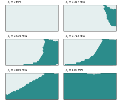
In the Settings window for 2D Plot Group, type Plastic Region, Mohr-Coulomb in the Label text field.
3
Locate the Data section. From the Dataset list, choose Mirror 2D 2.
Surface 1
1
In the Model Builder window, expand the Plastic Region, Mohr–Coulomb node, then click Surface 1.
2
In the Settings window for Surface, locate the Expression section.
3
In the Expression text field, type solid.epeGp>0.
4
Locate the Coloring and Style section. In the Number of bands text field, type 2.
5
Click to expand the Quality section. From the Evaluation settings list, choose Manual.
6
From the Resolution list, choose Custom.
7
In the Element refinement text field, type 2.
Plastic Region, Drucker–Prager
1
In the Model Builder window, under Results click Equivalent Plastic Strain (solid).
2
In the Settings window for 2D Plot Group, type Plastic Region, Drucker-Prager in the Label text field.
Surface 1
1
In the Model Builder window, expand the Plastic Region, Drucker–Prager node, then click Surface 1.
2
In the Settings window for Surface, locate the Expression section.
3
In the Expression text field, type solid.epeGp>0.
4
Locate the Coloring and Style section. In the Number of bands text field, type 2.
5
Locate the Quality section. From the Evaluation settings list, choose Manual.
6
From the Resolution list, choose Custom.
7
In the Element refinement text field, type 2.
8
Click the  Zoom Extents button in the Graphics toolbar.
Footing Pressure vs. Displacement
1
In the Results toolbar, click  1D Plot Group.
2
Drag and drop below Plastic Region, Mohr–Coulomb.
3
In the Settings window for 1D Plot Group, type Footing Pressure vs. Displacement in the Label text field.
4
Locate the Legend section. From the Position list, choose Lower right.
Point Graph 1
1
Right-click Footing Pressure vs. Displacement and choose Point Graph.
2
In the Settings window for Point Graph, locate the Data section.
3
From the Dataset list, choose Study: Drucker–Prager/Solution 1 (sol1).
4
5
Locate the y-Axis Data section. In the Expression text field, type abs(footing_pressure).
6
Select the Description checkbox. In the associated text field, type Footing pressure.
7
Locate the x-Axis Data section. From the Parameter list, choose Expression.
8
In the Expression text field, type abs(v).
9
Select the Description checkbox. In the associated text field, type Vertical displacement.
10
Click to expand the Legends section. Select the Show legends checkbox.
11
From the Legends list, choose Manual.
12
Point Graph 2
1
Right-click Point Graph 1 and choose Duplicate.
2
In the Settings window for Point Graph, locate the Data section.
3
From the Dataset list, choose Study: Mohr–Coulomb/Solution 2 (sol2).
4
Click to expand the Title section. From the Title type list, choose None.
5
Locate the Legends section. In the table, enter the following settings:
Footing Pressure vs. Displacement
1
In the Model Builder window, click Footing Pressure vs. Displacement.
2
In the Footing Pressure vs. Displacement toolbar, click  Plot.