PDF

Concrete Damage–Plasticity Material Tests
Introduction
This example shows the behavior of the coupled damage–plasticity model for concrete when subjected to different loading conditions. Several material tests that are commonly used to characterize concrete are set up for this purpose
For details on the coupled damage–plasticity material model, see the section Coupled Damage–Plasticity in the Structural Mechanics Module User’s Guide, and Ref. 1 and Ref. 2.
Model Definition
The Test material feature is used to test the material model when subjected to different loading conditions. Hence no specific geometry is required for the base component of the model. Concrete is, however, a so-called quasibrittle material which means that its response is size dependent, especially in tension. The size of the test specimen used by Test material is therefore important for the tests to give representative results. Here a characteristic size of 0.1 m is used.
In total six different tests are set up:
1
2
3
4
5
6
A generic set of material proprieties are used for the concrete, (see Table 1), but the model can be used to verify the model response for other properties as well. Note that these material properties are sufficient to define the model parameters of the coupled damage–plasticity model, but there are many more parameters available to modify the response of the material model that are here kept equal to their default value.
ν
σuc
σut
Gft
Results and Discussion
Figure 1 shows the results of the first two tests. The characteristic anisotropy of concrete in compression versus tension is clearly observable.
Figure 1: Stress versus strain for concrete subjected to monotonic uniaxial loading.
Results from the biaxial compression test are shown in Figure 2, which shows the stress in the main loading direction versus all three normal components of the strain tensor.
Figure 2: Stress versus strain for concrete subjected to monotonic biaxial compression.
Results from the isotropic compression test are shown in Figure 3, where it is clearly visible that the model response is ductile. The transition from a quasibrittle to a ductile response as the stress state goes toward isotropic compression is an important characteristic of concrete subjected to severe loading.
Figure 3: Stress versus strain for concrete subjected to monotonic isotropic compression.
Figure 4 and Figure 5 show results from the two cyclic tests. It is clearly visible how the response during cyclic loading deviates from the monotonic stress versus strain curve since there is irreversible deformation. In Figure 4 one can also note that all available plastic deformation occurs when the specimen is loaded in tension and starts to crack. Hence, there is no plastic hardening when the stress is reversed to compression; instead the response is “elastic” until softening starts.
.
Figure 4: Stress versus strain for concrete subjected to cyclic uniaxial loading going tension to compression and back to tension. The dotted black curve shows the stress versus strain for monotonic loading.
.
Figure 5: Stress versus strain for concrete subjected to cyclic uniaxial loading going from compression to tension. The dotted black curve shows the stress versus strain for monotonic loading.
References
1. P. Grassl and M. Jirásek, “Damage-plastic model for concrete failure,” Int. J. Solids Struct., vol. 43, pp. 7166–7196, 2006.
2. P. Grassl, D. Xenos, U. Nyström, R. Rempling, and K. Gylltoft, “CDPM2: A damage-plasticity approach to modelling the failure of concrete,” Int. J. Solids Struct., vol. 50, pp. 3805–3816, 2013.
Application Library path: Geomechanics_Module/Verification_Examples/concrete_damage_plasticity
Modeling Instructions
From the File menu, choose New.
New
In the New window, click  Model Wizard.
Model Wizard
1
In the Model Wizard window, click  3D.
2
In the Select Physics tree, select Structural Mechanics > Solid Mechanics (solid).
3
Click Add.
4
Geometry 1
Block 1 (blk1)
In the Geometry toolbar, click  Block.
Solid Mechanics (solid)
Linear Elastic Material 1
In the Model Builder window, under Component 1 (comp1) > Solid Mechanics (solid) click Linear Elastic Material 1.
Concrete 1
1
In the Physics toolbar, click  Attributes and choose Concrete.
2
In the Settings window for Concrete, locate the Concrete Model section.
3
From the Material model list, choose Coupled damage–plasticity.
Add Material
1
In the Materials toolbar, click  Add Material to open the Add Material window.
2
Go to the Add Material window.
3
In the tree, select Built-in > Concrete.
4
Click the Add to Component button in the window toolbar.
5
In the Materials toolbar, click  Add Material to close the Add Material window.
Materials
Concrete (mat1)
1
In the Settings window for Material, locate the Material Contents section.
2
Add a number of monotonic tests for different loading conditions.
Solid Mechanics (solid)
Monotonic Tests
1
In the Physics toolbar, click  Global and choose Test Material.
2
In the Settings window for Test Material, type Monotonic Tests in the Label text field.
3
4
Locate the Material Tests section. From the Specimen size list, choose User defined.
5
In the L text field, type 0.1[m].
6
Find the Tests subsection. In the λmin text field, type 1-5e-3.
7
In the λmax text field, type 1+1e-3.
8
Select the Biaxial test checkbox.
9
In the λmin text field, type 1-5e-3.
10
In the λmax text field, type 1.
11
In the β text field, type 0.5.
12
Select the Isotropic test checkbox.
13
In the λmin text field, type 1-1e-2.
14
Click Automated Model Setup in the upper-right corner of the Material Tests section. From the menu, choose Set up and Run Tests.
Set default units for result presentation.
Results
Preferred Units 1
1
In the Results toolbar, click  Configurations and choose Preferred Units.
2
In the Settings window for Preferred Units, locate the Units section.
3
Click  Add Physical Quantity.
4
In the Physical Quantity dialog, select Solid Mechanics > Stress tensor (N/m^2) in the tree.
5
6
In the Settings window for Preferred Units, locate the Units section.
7
8
Click  Add Physical Quantity.
9
In the Physical Quantity dialog, select General > Pressure (Pa) in the tree.
10
11
In the Settings window for Preferred Units, locate the Units section.
12
13
Click  Apply.
True Longitudinal Stress vs. True Longitudinal Strain (Uniaxial Test)
In the Model Builder window, expand the Results > Material Tests (Study: Monotonic Tests) node.
Point Graph 2
1
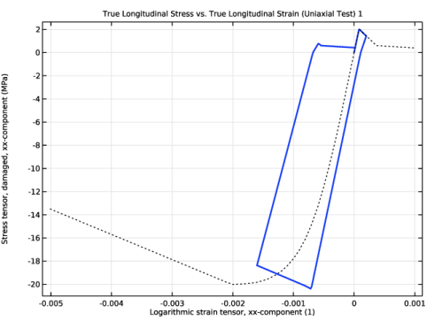
In the Model Builder window, expand the True Longitudinal Stress vs. True Longitudinal Strain (Uniaxial Test) node, then click Point Graph 2.
2
In the True Longitudinal Stress vs. True Longitudinal Strain (Uniaxial Test) toolbar, click  Plot.
Point Graph 1
1
In the Model Builder window, expand the Results > Material Tests (Study: Monotonic Tests) > True Longitudinal Stress vs. True Longitudinal Strain (Biaxial Test) node, then click Point Graph 1.
2
In the Settings window for Point Graph, click to expand the Legends section.
3
Select the Show legends checkbox.
4
From the Legends list, choose Manual.
5
Also plot the longitudinal stress versus the transverse and out-of-plane strain components.
Point Graph 2
1
Right-click Results > Material Tests (Study: Monotonic Tests) > True Longitudinal Stress vs. True Longitudinal Strain (Biaxial Test) > Point Graph 1 and choose Duplicate.
2
In the Settings window for Point Graph, locate the x-Axis Data section.
3
In the Expression text field, type solid1.elogyy.
4
Locate the Legends section. In the table, enter the following settings:
Point Graph 3
1
Right-click Point Graph 2 and choose Duplicate.
2
In the Settings window for Point Graph, locate the x-Axis Data section.
3
In the Expression text field, type solid1.elogzz.
4
Locate the Legends section. In the table, enter the following settings:
True Longitudinal Stress (Biaxial Test)
1
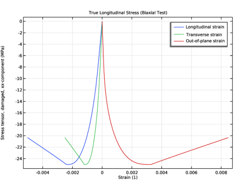
In the Model Builder window, under Results > Material Tests (Study: Monotonic Tests) click True Longitudinal Stress vs. True Longitudinal Strain (Biaxial Test).
2
In the Settings window for 1D Plot Group, type True Longitudinal Stress (Biaxial Test) in the Label text field.
3
Locate the Plot Settings section.
4
Select the x-axis label checkbox. In the associated text field, type Strain (1).
5
In the True Longitudinal Stress (Biaxial Test) toolbar, click  Plot.
Point Graph 1
1
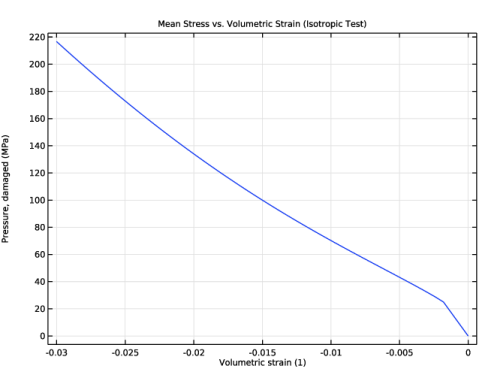
In the Model Builder window, expand the Mean Stress vs. Volumetric Strain (Isotropic Test) node, then click Point Graph 1.
2
In the Mean Stress vs. Volumetric Strain (Isotropic Test) toolbar, click  Plot.
Add a cyclic uniaxial test for the loading sequence: tension to compression to tension.
Global Definitions
Interpolation 1 (int1)
1
In the Home toolbar, click  Functions and choose Global > Interpolation.
2
In the Settings window for Interpolation, locate the Definition section.
3
Solid Mechanics (solid)
Cyclic Test 1
1
In the Physics toolbar, click  Global and choose Test Material.
2
In the Settings window for Test Material, type Cyclic Test 1 in the Label text field.
3
4
Locate the Material Tests section. From the Specimen size list, choose User defined.
5
In the L text field, type 0.1[m].
6
From the Test setup list, choose User defined.
7
In the paramax text field, type 3.
8
In the Np text field, type 300.
9
Find the Tests subsection. In the λ text field, type 1+int1(para).
10
Click Automated Model Setup in the upper-right corner of the Material Tests section. From the menu, choose Set up and Run Tests.
Add the uniaxial stress-strain curve from the monotonic test as a reference.
Results
Point Graph 1, Point Graph 2
1
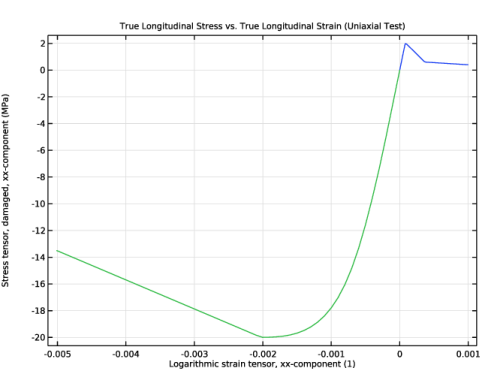
In the Model Builder window, under Results > Material Tests (Study: Monotonic Tests) > True Longitudinal Stress vs. True Longitudinal Strain (Uniaxial Test), Ctrl-click to select Point Graph 1 and Point Graph 2.
2
True Longitudinal Stress vs. True Longitudinal Strain (Uniaxial Test) 1
1
In the Model Builder window, expand the Results > Material Tests (Study: Cyclic Test 1) node.
2
Right-click True Longitudinal Stress vs. True Longitudinal Strain (Uniaxial Test) 1 and choose Paste Multiple Items.
Point Graph 2, Point Graph 3
1
In the Settings window for Point Graph, click to expand the Coloring and Style section.
2
Find the Line style subsection. From the Line list, choose Dotted.
3
From the Color list, choose Black.
Point Graph 3
1
In the Model Builder window, click Point Graph 3.
2
In the Settings window for Point Graph, locate the Coloring and Style section.
3
Find the Line style subsection. From the Line list, choose Dotted.
4
From the Color list, choose Black.
Point Graph 1
1
In the Model Builder window, click Point Graph 1.
2
In the Settings window for Point Graph, locate the Coloring and Style section.
3
From the Width list, choose 2.
4
In the True Longitudinal Stress vs. True Longitudinal Strain (Uniaxial Test) 1 toolbar, click  Plot.
Add a cyclic uniaxial test for the loading sequence: compression to tension.
Global Definitions
Interpolation 2 (int2)
1
In the Home toolbar, click  Functions and choose Global > Interpolation.
2
In the Settings window for Interpolation, locate the Definition section.
3
Solid Mechanics (solid)
Cyclic Test 2
1
In the Physics toolbar, click  Global and choose Test Material.
2
In the Settings window for Test Material, type Cyclic Test 2 in the Label text field.
3
4
Locate the Material Tests section. From the Specimen size list, choose User defined.
5
In the L text field, type 0.1[m].
6
From the Test setup list, choose User defined.
7
In the paramax text field, type 2.
8
In the Np text field, type 200.
9
Find the Tests subsection. In the λ text field, type 1+int2(para).
10
Click Automated Model Setup in the upper-right corner of the Material Tests section. From the menu, choose Set up and Run Tests.
Results
Point Graph 2, Point Graph 3
1
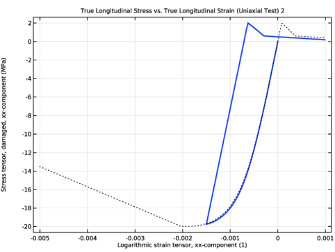
In the Model Builder window, under Results > Material Tests (Study: Cyclic Test 1) > True Longitudinal Stress vs. True Longitudinal Strain (Uniaxial Test) 1, Ctrl-click to select Point Graph 2 and Point Graph 3.
2
True Longitudinal Stress vs. True Longitudinal Strain (Uniaxial Test) 2
1
In the Model Builder window, expand the Results > Material Tests (Study: Cyclic Test 2) node.
2
Right-click True Longitudinal Stress vs. True Longitudinal Strain (Uniaxial Test) 2 and choose Paste Multiple Items.
Point Graph 1
1
In the Settings window for Point Graph, locate the Coloring and Style section.
2
From the Width list, choose 2.
3
In the True Longitudinal Stress vs. True Longitudinal Strain (Uniaxial Test) 2 toolbar, click  Plot.