|
|
|
|
•
|
|
•
|
|
•
|
|
•
|
|
•
|


|
1
|
|
2
|
|
3
|
Click Add.
|
|
4
|
|
5
|
Click Add.
|
|
6
|
Click
|
|
7
|
|
8
|
Click
|
|
1
|
|
2
|
|
3
|
Click
|
|
4
|
Browse to the model’s Application Libraries folder and double-click the file concrete_beam_parameters.txt.
|
|
1
|
|
2
|
|
3
|
|
4
|
|
5
|
|
6
|
Click to expand the Layers section. In the table, enter the following settings:
|
|
1
|
|
2
|
|
3
|
|
4
|
|
5
|
|
6
|
|
7
|
|
8
|
|
9
|
|
10
|
Locate the Selections of Resulting Entities section. Find the Cumulative selection subsection. Click New.
|
|
11
|
|
12
|
Click OK.
|
|
1
|
|
2
|
|
3
|
|
4
|
|
5
|
|
1
|
|
2
|
|
3
|
|
4
|
|
5
|
|
6
|
|
7
|
|
8
|
Locate the Selections of Resulting Entities section. Find the Cumulative selection subsection. Click New.
|
|
9
|
|
10
|
Click OK.
|
|
1
|
|
2
|
|
3
|
|
4
|
|
5
|
|
1
|
|
3
|
|
4
|
|
5
|
Click
|
|
6
|
|
7
|
Click
|
|
1
|
|
2
|
|
3
|
|
4
|
Clear the Create pairs checkbox.
|
|
1
|
|
2
|
|
3
|
|
1
|
|
2
|
|
1
|
|
2
|
|
3
|
|
4
|
|
5
|
In the Add dialog, in the Selections to add list, choose Bars Inside Domain and Bars on Symmetry Plane.
|
|
6
|
Click OK.
|
|
1
|
|
2
|
|
3
|
|
4
|
|
6
|
|
1
|
In the Model Builder window, under Component 1 (comp1) > Solid Mechanics (solid) click Linear Elastic Material 1.
|
|
1
|
|
2
|
|
3
|
|
1
|
|
1
|
|
3
|
In the Settings window for Rigid Connector, locate the Prescribed Displacement at Center of Rotation section.
|
|
4
|
Select the Prescribed in y direction checkbox.
|
|
5
|
Select the Prescribed in z direction checkbox.
|
|
6
|
|
7
|
Select the Constrain rotation around x-axis checkbox.
|
|
8
|
Select the Constrain rotation around z-axis checkbox.
|
|
1
|
|
3
|
|
4
|
|
5
|
|
6
|
In the Show More Options dialog, in the tree, select the checkbox for the node Physics > Equation Contributions.
|
|
7
|
Click OK.
|
|
1
|
|
2
|
|
4
|
|
5
|
|
6
|
|
7
|
Click OK.
|
|
8
|
|
9
|
Click
|
|
10
|
|
11
|
|
12
|
Click OK.
|
|
1
|
|
2
|
|
3
|
|
1
|
|
2
|
|
3
|
|
1
|
|
2
|
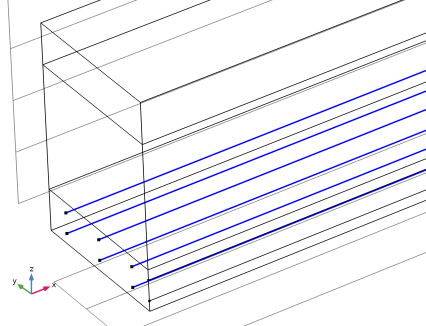
In the Settings window for Embedded Reinforcement, locate the Edge Selection, Embedded Structure section.
|
|
3
|
|
1
|
|
2
|
Go to the Add Material window.
|
|
3
|
|
4
|
Click the Add to Component button in the window toolbar.
|
|
5
|
|
6
|
Click the Add to Component button in the window toolbar.
|
|
7
|
|
1
|
|
1
|
|
2
|
|
3
|
|
4
|
|
5
|
Locate the Material Contents section. In the table, enter the following settings:
|
|
1
|
|
2
|
|
3
|
|
1
|
|
2
|
|
3
|
|
1
|
|
1
|
|
3
|
|
4
|
|
1
|
|
3
|
|
4
|
|
1
|
|
2
|
|
3
|
|
4
|
|
5
|
|
1
|
|
2
|
|
1
|
|
2
|
|
3
|
Select the Modify model configuration for study step checkbox.
|
|
4
|
In the tree, select Component 1 (comp1) > Solid Mechanics (solid) > Linear Elastic Material 1 > Concrete 1.
|
|
5
|
Right-click and choose Disable.
|
|
6
|
|
7
|
Click
|
|
8
|
|
9
|
Click
|
|
10
|
|
11
|
Click
|
|
1
|
|
2
|
|
3
|
In the Model Builder window, expand the Without Bars > Solver Configurations > Solution 1 (sol1) > Stationary Solver 1 node.
|
|
4
|
Right-click Without Bars > Solver Configurations > Solution 1 (sol1) > Stationary Solver 1 > Parametric 1 and choose Stop Condition.
|
|
5
|
|
6
|
Click
|
|
8
|
|
9
|
Clear the Add information checkbox.
|
|
10
|
|
1
|
|
2
|
|
3
|
|
4
|
|
1
|
|
2
|
|
3
|
|
4
|
|
1
|
|
2
|
|
3
|
Click
|
|
4
|
|
5
|
Click OK.
|
|
6
|
|
8
|
Click
|
|
1
|
|
2
|
|
3
|
|
4
|
|
1
|
|
2
|
|
3
|
|
1
|
|
2
|
Go to the Add Study window.
|
|
3
|
|
4
|
Click the Add Study button in the window toolbar.
|
|
5
|
|
1
|
|
2
|
Select the Modify model configuration for study step checkbox.
|
|
3
|
In the tree, select Component 1 (comp1) > Solid Mechanics (solid) > Linear Elastic Material 1 > Concrete 1.
|
|
4
|
Click
|
|
5
|
|
6
|
Click
|
|
1
|
|
2
|
|
3
|
In the Model Builder window, expand the Study 2 > Solver Configurations > Solution 2 (sol2) > Stationary Solver 1 node.
|
|
4
|
Right-click Study 2 > Solver Configurations > Solution 2 (sol2) > Stationary Solver 1 > Parametric 1 and choose Stop Condition.
|
|
5
|
|
6
|
Click
|
|
8
|
|
9
|
Clear the Add information checkbox.
|
|
10
|
|
11
|
|
12
|
|
1
|
|
2
|
|
3
|
|
4
|
|
5
|
|
1
|
|
2
|
|
3
|
|
4
|
|
1
|
|
2
|
|
3
|
|
4
|
|
1
|
|
2
|
|
3
|
|
1
|
|
2
|
|
3
|
|
4
|
|
1
|
|
2
|
|
3
|
|
4
|
|
5
|
|
6
|
|
1
|
|
2
|
Go to the Result Templates window.
|
|
3
|
|
4
|
Click the Add Result Template button in the window toolbar.
|
|
5
|
|
1
|
|
2
|
|
3
|
|
1
|
|
2
|
|
3
|
|
4
|
|
5
|
|
6
|
|
7
|
|
1
|
In the Model Builder window, under Results, Ctrl-click to select Stress 2, Stress in Bars 2, and Force in Bars 2.
|
|
2
|
Right-click and choose Group.
|
|
1
|
|
2
|
Go to the Add Study window.
|
|
3
|
|
4
|
Click the Add Study button in the window toolbar.
|
|
5
|
|
1
|
|
2
|
Select the Auxiliary sweep checkbox.
|
|
3
|
Click
|
|
5
|
|
6
|
|
7
|
Clear the Generate default plots checkbox.
|
|
1
|
|
2
|
|
3
|
In the Model Builder window, expand the Study 3 > Solver Configurations > Solution 3 (sol3) > Stationary Solver 1 node, then click Parametric 1.
|
|
4
|
|
5
|
|
6
|
Right-click Study 3 > Solver Configurations > Solution 3 (sol3) > Stationary Solver 1 > Parametric 1 and choose Stop Condition.
|
|
7
|
|
8
|
Click
|
|
10
|
|
11
|
Clear the Add information checkbox.
|
|
12
|
|
13
|
|
14
|
|
1
|
|
2
|
|
3
|
|
4
|
|
5
|
|
1
|
|
2
|
|
3
|
|
4
|
|
1
|
|
2
|
|
1
|
|
2
|
|
3
|
|
4
|
Click
|
|
5
|
|
1
|
|
2
|
|
3
|
|
4
|
Click
|
|
1
|
|
2
|
|
3
|
|
4
|
|
5
|
Click
|
|
1
|
|
2
|
|
3
|
|
4
|
|
1
|
|
2
|
|
3
|
|
4
|
|
5
|
|
6
|
|
1
|
|
2
|
|
3
|
Click
|
|
4
|
|
1
|
|
2
|
|
3
|
|
4
|
|
5
|
|
6
|
|
7
|
|
8
|
In the Show More Options dialog, in the tree, select the checkbox for the node Physics > Advanced Physics Options.
|
|
9
|
Click OK.
|
|
1
|
|
2
|
|
3
|
|
1
|
|
2
|
|
1
|
|
2
|
|
1
|
|
2
|
Go to the Add Study window.
|
|
3
|
|
4
|
Click the Add Study button in the window toolbar.
|
|
5
|
|
1
|
|
2
|
|
3
|
Click
|
|
1
|
|
2
|
|
3
|
Select the Modify model configuration for study step checkbox.
|
|
4
|
|
5
|
|
6
|
|
7
|
|
8
|
|
9
|
Click
|
|
11
|
|
12
|
|
13
|
Clear the Generate default plots checkbox.
|
|
1
|
|
2
|
|
3
|
In the Model Builder window, expand the Study 4 > Solver Configurations > Solution 4 (sol4) > Stationary Solver 1 node.
|
|
4
|
Right-click Study 4 > Solver Configurations > Solution 4 (sol4) > Stationary Solver 1 > Parametric 1 and choose Stop Condition.
|
|
5
|
|
6
|
Click
|
|
8
|
|
9
|
Clear the Add information checkbox.
|
|
10
|
|
11
|
|
12
|
|
1
|
|
2
|
|
3
|
|
4
|
|
5
|
|
1
|
|
2
|
|
3
|
|
4
|
|
1
|
|
2
|
|
1
|
|
2
|
|
3
|
|
1
|
|
2
|
|
3
|
|
4
|
Click
|
|
5
|
|
1
|
|
2
|
|
3
|
|
4
|
Click
|
|
1
|
|
2
|
|
3
|
|
4
|
|
5
|
Click
|
|
1
|
|
2
|
|
3
|
|
4
|
|
1
|
|
2
|
|
3
|
|
4
|
|
5
|
|
6
|
|
1
|
|
2
|
Clear the Plot dataset edges checkbox.
|
|
3
|
Click
|
|
4
|
|
1
|
|
2
|
|
3
|
|
4
|
|
1
|
|
2
|
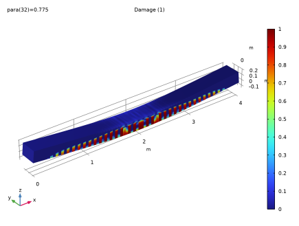
In the Settings window for Surface, click Replace Expression in the upper-right corner of the Expression section. From the menu, choose Component 1 (comp1) > Solid Mechanics > Damage > solid.eeqGp - Equivalent strain - 1.
|
|
3
|
|
4
|
|
5
|
|
6
|
|
7
|
|
8
|
|
1
|
|
2
|
Clear the Plot dataset edges checkbox.
|
|
3
|
Click
|
|
4
|
|
1
|
|
2
|
|
4
|
Click
|
|
6
|
|
7
|
|
8
|
Locate the Fiber Model section. From the Efiber list, choose User defined. In the associated text field, type mat1.Enu.E+mat2.Enu.E.
|
|
1
|
|
2
|
Go to the Add Study window.
|
|
3
|
|
4
|
Find the Physics interfaces in study subsection. In the table, clear the Solve checkbox for Truss (truss).
|
|
5
|
Find the Multiphysics couplings in study subsection. In the table, clear the Solve checkbox for Embedded Reinforcement 1 (ere1).
|
|
6
|
Click the Add Study button in the window toolbar.
|
|
7
|
|
1
|
|
2
|
Select the Modify model configuration for study step checkbox.
|
|
3
|
In the tree, select Component 1 (comp1) > Solid Mechanics (solid) > Linear Elastic Material 1 > Concrete 2.
|
|
4
|
Click
|
|
5
|
In the tree, select Component 1 (comp1) > Solid Mechanics (solid) > Linear Elastic Material 1 > Concrete 1.
|
|
6
|
Click
|
|
7
|
|
8
|
Click
|
|
1
|
|
2
|
|
3
|
In the Model Builder window, expand the Study 5 > Solver Configurations > Solution 7 (sol7) > Stationary Solver 1 node.
|
|
4
|
Right-click Study 5 > Solver Configurations > Solution 7 (sol7) > Stationary Solver 1 > Parametric 1 and choose Stop Condition.
|
|
5
|
|
6
|
Click
|
|
8
|
|
9
|
Clear the Add information checkbox.
|
|
10
|
|
11
|
|
12
|
|
1
|
|
2
|
|
3
|
|
1
|
|
2
|
|
3
|
|
1
|
|
2
|
|
3
|
|
4
|
|
5
|
|
1
|
|
2
|
|
1
|
|
2
|
Go to the Result Templates window.
|
|
3
|
In the tree, select With Fibers/Solution 7 (sol7) > Solid Mechanics > Fibers (solid) > Fiber, Linear Elastic Material 1 (solid).
|
|
4
|
Click the Add Result Template button in the window toolbar.
|
|
5
|
|
1
|
|
2
|
|
3
|
|
4
|
|
1
|
|
2
|
|
1
|
|
2
|
|
3
|
|
4
|
|
1
|
|
2
|
|
3
|
|
4
|
|
1
|
|
2
|
Right-click and choose Group.
|
|
1
|
|
2
|
|
3
|
|
4
|
|
5
|
|
6
|
Locate the Plot Settings section.
|
|
7
|
|
8
|
|
9
|
|
1
|
|
2
|
|
3
|
|
4
|
|
6
|
|
7
|
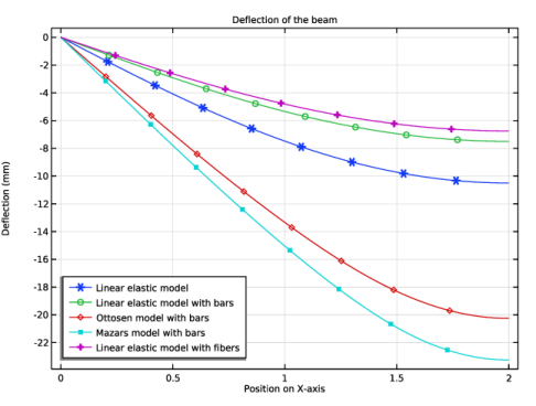
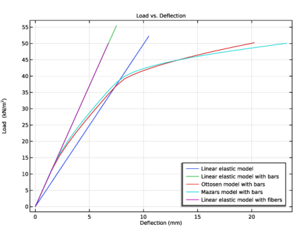
Click Replace Expression in the upper-right corner of the y-Axis Data section. From the menu, choose Component 1 (comp1) > Solid Mechanics > Displacement > Displacement field - m > w - Displacement field, Z-component.
|
|
8
|
|
9
|
|
10
|
Click to expand the Coloring and Style section. Find the Line markers subsection. From the Marker list, choose Cycle.
|
|
11
|
|
12
|
|
13
|
|
1
|
|
2
|
|
3
|
|
4
|
Locate the Legends section. In the table, enter the following settings:
|
|
1
|
In the Model Builder window, under Results > Deflection right-click Line Graph 1 and choose Duplicate.
|
|
2
|
|
3
|
|
4
|
Locate the Legends section. In the table, enter the following settings:
|
|
1
|
|
2
|
|
3
|
|
4
|
Locate the Legends section. In the table, enter the following settings:
|
|
1
|
|
2
|
|
3
|
|
4
|
Locate the Legends section. In the table, enter the following settings:
|
|
5
|
|
6
|
|
7
|
|
1
|
|
2
|
|
3
|
|
4
|
|
5
|
|
6
|
Locate the Plot Settings section.
|
|
7
|
|
8
|
|
9
|
|
1
|
|
2
|
|
3
|
|
4
|
|
5
|
|
7
|
|
8
|
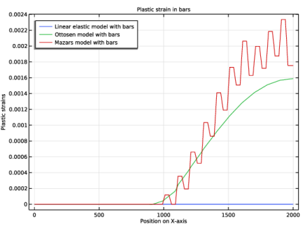
Click Replace Expression in the upper-right corner of the y-Axis Data section. From the menu, choose Component 1 (comp1) > Truss > Strain > truss.epnGp - Plastic axial strain - 1.
|
|
9
|
|
10
|
|
11
|
|
12
|
|
13
|
|
1
|
|
2
|
|
3
|
|
4
|
Locate the Legends section. In the table, enter the following settings:
|
|
1
|
In the Model Builder window, under Results > Plastic Strains right-click Line Graph 1 and choose Duplicate.
|
|
2
|
|
3
|
|
4
|
Locate the Legends section. In the table, enter the following settings:
|
|
5
|
|
6
|
|
1
|
|
2
|
|
3
|
|
4
|
|
5
|
Locate the Plot Settings section.
|
|
6
|
|
7
|
|
8
|
|
1
|
|
2
|
|
3
|
|
4
|
Locate the y-Axis Data section. In the table, enter the following settings:
|
|
5
|
|
6
|
|
7
|
|
8
|
Click to expand the Coloring and Style section.
|
|
1
|
|
2
|
|
3
|
|
4
|
Locate the y-Axis Data section. In the table, enter the following settings:
|
|
1
|
In the Model Builder window, under Results > Load vs. Deflection right-click Global 1 and choose Duplicate.
|
|
2
|
|
3
|
|
4
|
Locate the y-Axis Data section. In the table, enter the following settings:
|
|
1
|
|
2
|
|
3
|
|
4
|
Locate the y-Axis Data section. In the table, enter the following settings:
|
|
1
|
|
2
|
|
3
|
|
4
|
Locate the y-Axis Data section. In the table, enter the following settings:
|
|
5
|
|
6
|
|
1
|
|
2
|
|
3
|
In the tree, select Component 1 (comp1) > Solid Mechanics (solid) > Linear Elastic Material 1 > Concrete 2.
|
|
4
|
Click
|
|
5
|
In the tree, select Component 1 (comp1) > Solid Mechanics (solid) > Linear Elastic Material 1 > Fiber 1.
|
|
6
|
Click
|
|
1
|
|
2
|
|
3
|
In the tree, select Component 1 (comp1) > Solid Mechanics (solid) > Linear Elastic Material 1 > Concrete 2.
|
|
4
|
Click
|
|
5
|
In the tree, select Component 1 (comp1) > Solid Mechanics (solid) > Linear Elastic Material 1 > Fiber 1.
|
|
6
|
Click
|
|
1
|
|
2
|
|
3
|
Select the Modify model configuration for study step checkbox.
|
|
4
|
In the tree, select Component 1 (comp1) > Solid Mechanics (solid) > Linear Elastic Material 1 > Concrete 2.
|
|
5
|
Click
|
|
6
|
In the tree, select Component 1 (comp1) > Solid Mechanics (solid) > Linear Elastic Material 1 > Fiber 1.
|
|
7
|
Click
|
|
1
|
|
2
|
|
3
|
In the tree, select Component 1 (comp1) > Solid Mechanics (solid) > Linear Elastic Material 1 > Fiber 1.
|
|
4
|
Click
|