PDF

Block Verification
Introduction
This example shows how to set up a compression test on a prestressed soil sample. Due to a simple stress state, it is possible to determine the vertical yield stress analytically. The soil sample is modeled with soil plasticity and the Mohr–Coulomb criterion.
Model Definition
In this example, we consider a block of soil of 1 m length on each side. The soil is pressed from the sides by boundary loads in the x and y directions, and from the top by a prescribed displacement.
Figure 1: Dimensions, boundary conditions, and loads for the test.
Elastic Properties
The soil properties are taken from standard clay.
Young’s modulus, E = 207 MPa, and Poisson’s ratio ν = 0.3.
Soil Plasticity
Cohesion c = 70 kPa, and angle of internal friction .
Constraints and Loads
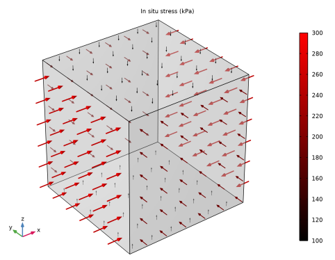
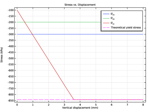
The in situ stress is prescribed via the External Stress node, it is 300 kPa, 200 kPa, and 100 kPa in the x, y, and z directions, respectively. The in situ stress components are shown in Figure 2.
Figure 2: In situ stress applied on the surface of the block.
Results and Discussion
The cube of soil experiences a homogeneous stress state, as shown by the von Mises stress distribution in Figure 3.
Figure 3: Equivalent stress and deformation in the soil sample after applying 8 mm displacement from the top.
The stress increases with the compression of the block, as shown in Figure 4.
Figure 4: Equivalent stress with compression displacement of 0 mm, 2 mm, 6 mm, and 8 mm.
From the Mohr circle, the Mohr–Coulomb criterion can be written in terms of the biggest and smallest principal stress:
Since stress in the y direction is the largest principal stress and the stress in the z direction is the smallest principal stress at the onset of yielding, its analytical value can be obtained. Manipulation of the above formula gives
(1)
The stresses history together with the analytical value of the stress in the z direction at the onset of yielding is shown in Figure 5. Plastic yielding is reached after a deflection of about 3.5 mm.
Figure 5: This plot shows how the soil sample behaves elastically until it reaches the yield surface at the compressive meridian.
Application Library path: Geomechanics_Module/Verification_Examples/block_verification
Modeling Instructions
From the File menu, choose New.
New
In the New window, click  Model Wizard.
Model Wizard
1
In the Model Wizard window, click  3D.
2
In the Select Physics tree, select Structural Mechanics > Solid Mechanics (solid).
3
Click Add.
4
Click  Study.
5
In the Select Study tree, select General Studies > Stationary.
6
Global Definitions
Parameters 1
1
In the Model Builder window, under Global Definitions click Parameters 1.
2
In the Settings window for Parameters, locate the Parameters section.
3
In situ stresses are set with negative sign to fit the structural mechanics convention which assumes negative stresses in compression, and positive in tension.
Geometry 1
Block 1 (blk1)
1
In the Model Builder window, expand the Component 1 (comp1) > Geometry 1 node.
2
Right-click Geometry 1 and choose Block.
3
In the Settings window for Block, click  Build All Objects.
The geometry consists of a simple unit block.
Definitions
Integration 1 (intop1)
1
In the Definitions toolbar, click  Nonlocal Couplings and choose Integration.
2
In the Settings window for Integration, locate the Source Selection section.
3
From the Geometric entity level list, choose Boundary.
4
Variables 1
1
In the Model Builder window, right-click Definitions and choose Variables.
2
In the Settings window for Variables, locate the Variables section.
3
Solid Mechanics (solid)
Linear Elastic Material 1
In the Model Builder window, under Component 1 (comp1) > Solid Mechanics (solid) click Linear Elastic Material 1.
Soil Plasticity 1
1
In the Physics toolbar, click  Attributes and choose Soil Plasticity.
2
In the Settings window for Soil Plasticity, locate the Soil Plasticity Model section.
3
From the Ff list, choose Mohr–Coulomb.
The MohrCoulomb criterion is used to define yield surface.
Linear Elastic Material 1
In the Model Builder window, click Linear Elastic Material 1.
External Stress 1
1
In the Physics toolbar, click  Attributes and choose External Stress.
Choose the In situ option in order to apply the in situ stresses.
2
In the Settings window for External Stress, locate the External Stress section.
3
From the Stress input list, choose In situ stress.
4
5
Specify the σins matrix as
Roller 1
1
In the Physics toolbar, click  Boundaries and choose Roller.
2
Prescribed Displacement 1
1
In the Physics toolbar, click  Boundaries and choose Prescribed Displacement.
2
3
In the Settings window for Prescribed Displacement, locate the Prescribed Displacement section.
4
From the Displacement in z direction list, choose Prescribed.
5
In the u0z text field, type -Disp.
Materials
Material 1 (mat1)
1
In the Model Builder window, under Component 1 (comp1) right-click Materials and choose Blank Material.
2
In the Settings window for Material, locate the Material Contents section.
3
Mesh 1
Mapped 1
1
In the Mesh toolbar, click  More Generators and choose Mapped.
2
Swept 1
In the Mesh toolbar, click  Swept.
Size
1
In the Model Builder window, click Size.
2
In the Settings window for Size, locate the Element Size section.
3
From the Predefined list, choose Extra coarse.
4
Click  Build All.
Study 1
Step 1: Stationary
Set up an auxiliary continuation sweep for the Disp parameter.
1
In the Model Builder window, under Study 1 click Step 1: Stationary.
2
In the Settings window for Stationary, click to expand the Study Extensions section.
3
Select the Auxiliary sweep checkbox.
4
5
6
In the Study toolbar, click  Compute.
Set default units for result presentation.
Results
Preferred Units 1
1
In the Results toolbar, click  Configurations and choose Preferred Units.
2
In the Settings window for Preferred Units, locate the Units section.
3
Click  Add Physical Quantity.
4
In the Physical Quantity dialog, select Solid Mechanics > Stress tensor (N/m^2) in the tree.
5
6
In the Settings window for Preferred Units, locate the Units section.
7
8
Select the Apply conversions to expressions with the same dimensions checkbox.
9
Click  Apply.
Volume 1
1
In the Model Builder window, expand the Stress (solid) node, then click Volume 1.
2
In the Stress (solid) toolbar, click  Plot.
Stress (solid)
The default plot shows uniform stress (Figure 3). Modify it to show the von Mises stress at different stages of uniaxial compression, (Figure 4).
1
In the Model Builder window, click Stress (solid).
2
In the Settings window for 3D Plot Group, click to expand the Title section.
3
From the Title type list, choose Custom.
4
Find the Solution subsection. Clear the Solution checkbox.
5
Locate the Color Legend section. From the Position list, choose Bottom.
Deformation
1
In the Model Builder window, expand the Volume 1 node.
2
Right-click Deformation and choose Delete.
Solution Array 1
1
Right-click Volume 1 and choose Solution Array.
2
In the Settings window for Solution Array, locate the Data section.
3
From the Parameter selection (Disp) list, choose From list.
4
In the Parameter values (Disp (mm)) list, choose 0, 2, 6, and 8.
Arrow Surface 1
1
In the Model Builder window, right-click Stress (solid) and choose Arrow Surface.
2
In the Settings window for Arrow Surface, locate the Expression section.
3
In the X-component text field, type 0.
4
In the Y-component text field, type 0.
5
In the Z-component text field, type Forcez.
6
Click to expand the Title section. From the Title type list, choose None.
7
Locate the Arrow Positioning section. In the Number of arrows text field, type 40.
8
Locate the Coloring and Style section. From the Arrow base list, choose Head.
9
From the Color list, choose Custom.
10
11
Click Define custom colors.
12
13
Click Add to custom colors.
14
Click Show color palette only or OK on the cross-platform desktop.
15
Select the Scale factor checkbox. In the associated text field, type 4E-4.
16
Click to expand the Plot Array section. Select the Manual indexing checkbox.
Selection 1
1
Right-click Arrow Surface 1 and choose Selection.
2
Solution Array 1
1
In the Model Builder window, right-click Arrow Surface 1 and choose Solution Array.
2
In the Settings window for Solution Array, locate the Data section.
3
From the Parameter selection (Disp) list, choose From list.
4
In the Parameter values (Disp (mm)) list, choose 0, 2, 6, and 8.
Stress (solid)
1
In the Model Builder window, under Results click Stress (solid).
2
In the Settings window for 3D Plot Group, click to expand the Plot Array section.
3
In the Relative padding text field, type 1.
Table Annotation 1
1
In the Stress (solid) toolbar, click  More Plots and choose Table Annotation.
2
In the Settings window for Table Annotation, locate the Data section.
3
From the Source list, choose Local table.
4
5
Select the LaTeX markup checkbox.
6
Locate the Coloring and Style section. Clear the Show point checkbox.
Stress (solid)
1
Click the  Show Grid button in the Graphics toolbar.
2
In the Model Builder window, click Stress (solid).
3
In the Settings window for 3D Plot Group, locate the Plot Settings section.
4
From the View list, choose New view.
5
In the Stress (solid) toolbar, click  Plot.
Add a 1D plot to show the evolution of the stress-tensor components versus the displacement at the top surface.
Stress vs. Displacement
1
In the Results toolbar, click  1D Plot Group.
2
In the Settings window for 1D Plot Group, type Stress vs. Displacement in the Label text field.
3
Click to expand the Title section. From the Title type list, choose Label.
4
Locate the Plot Settings section.
5
Select the x-axis label checkbox. In the associated text field, type Vertical displacement (mm).
6
Select the y-axis label checkbox. In the associated text field, type Stress (kPa).
Point Graph 1
1
Right-click Stress vs. Displacement and choose Point Graph.
2
3
In the Settings window for Point Graph, click Replace Expression in the upper-right corner of the y-Axis Data section. From the menu, choose Component 1 (comp1) > Solid Mechanics > Stress > Stress tensor (spatial frame) - N/m² > solid.sGpxx - Stress tensor, xx-component.
4
Locate the x-Axis Data section. From the Parameter list, choose Expression.
5
In the Expression text field, type Disp.
6
From the Unit list, choose mm.
7
Click to expand the Coloring and Style section. Click to expand the Legends section. Select the Show legends checkbox.
8
From the Legends list, choose Manual.
9
10
In the Stress vs. Displacement toolbar, click  Plot.
Point Graph 2
1
Right-click Point Graph 1 and choose Duplicate.
2
In the Settings window for Point Graph, click Replace Expression in the upper-right corner of the y-Axis Data section. From the menu, choose Component 1 (comp1) > Solid Mechanics > Stress > Stress tensor (spatial frame) - N/m² > solid.sGpyy - Stress tensor, yy-component.
3
In the Stress vs. Displacement toolbar, click  Plot.
4
Locate the Legends section. In the table, enter the following settings:
Point Graph 3
1
In the Model Builder window, under Results > Stress vs. Displacement right-click Point Graph 1 and choose Duplicate.
2
In the Settings window for Point Graph, click Replace Expression in the upper-right corner of the y-Axis Data section. From the menu, choose Component 1 (comp1) > Solid Mechanics > Stress > Stress tensor (spatial frame) - N/m² > solid.sGpzz - Stress tensor, zz-component.
3
In the Stress vs. Displacement toolbar, click  Plot.
4
Locate the Legends section. In the table, enter the following settings:
Point Graph 4
1
Right-click Point Graph 1 and choose Duplicate.
2
In the Settings window for Point Graph, locate the y-Axis Data section.
3
In the Expression text field, type szz_th.
4
Locate the Coloring and Style section. Find the Line style subsection. From the Line list, choose Dashed.
5
From the Color list, choose Magenta.
6
Locate the Legends section. In the table, enter the following settings:
Stress vs. Displacement
1
In the Model Builder window, click Stress vs. Displacement.
2
In the Stress vs. Displacement toolbar, click  Plot.
Finally, plot the in situ stress on the boundaries to reproduce Figure 2.
In Situ Stress
1
In the Results toolbar, click  3D Plot Group.
2
In the Settings window for 3D Plot Group, type In Situ Stress in the Label text field.
3
Locate the Title section. From the Title type list, choose Manual.
4
In the Title text area, type In situ stress (kPa).
5
Clear the Parameter indicator text field.
Volume 1
1
In the In Situ Stress toolbar, click  Volume.
2
In the Settings window for Volume, locate the Expression section.
3
In the Expression text field, type 1.
4
Locate the Coloring and Style section. From the Coloring list, choose Uniform.
5
From the Color list, choose Gray.
Transparency 1
1
In the In Situ Stress toolbar, click  Transparency.
2
In the Settings window for Transparency, locate the Transparency section.
3
Find the Transparency subsection. Set the Transparency value to 0.7.
In Situ Stress
In the Model Builder window, under Results click In Situ Stress.
Arrow Surface 1
1
In the In Situ Stress toolbar, click  Arrow Surface.
2
In the Settings window for Arrow Surface, locate the Expression section.
3
In the X-component text field, type solid.SinsXX*solid.nX+solid.SinsXY*solid.nY+solid.SinsXZ*solid.nZ.
4
In the Y-component text field, type solid.SinsXY*solid.nX+solid.SinsYY*solid.nY+solid.SinsYZ*solid.nZ.
5
In the Z-component text field, type solid.SinsXZ*solid.nX+solid.SinsXZ*solid.nY+solid.SinsZZ*solid.nZ.
6
Locate the Coloring and Style section. From the Arrow base list, choose Head.
Color Expression 1
1
In the In Situ Stress toolbar, click  Color Expression.
2
In the Settings window for Color Expression, locate the Expression section.
3
From the Color data list, choose Arrow length.
4
Locate the Coloring and Style section. From the Coloring list, choose Gradient.
5
From the Top color list, choose Red.
6
In the In Situ Stress toolbar, click  Plot.