|
|
|
|
•
|
Darcy’s Law, solving for the liquid pressure in the GDEs
|
|
•
|
Laminar Flow, solving for the liquid pressure and velocity field in the channels
|
|
•
|
Phase Transport, solving for the gas phase volume fraction in the gas-liquid two-phase mixture
|
|
•
|
Multiphase Flow in Porous Media, coupling Darcy’s law and Phase Transport in the GDEs
|
|
•
|
Free and Porous Media Flow Coupling, defining the boundary between the Laminar Flow and Darcy’s Law domains
|
|
•
|
Mixture Model, coupling Laminar Flow and Phase Transport in the channels
|


|
1
|
|
2
|
|
3
|
Click Add.
|
|
4
|
In the Select Physics tree, select Fluid Flow > Porous Media and Subsurface Flow > Multiphase Free and Porous Media Flow.
|
|
5
|
Click Add.
|
|
6
|
|
7
|
Click Add.
|
|
8
|
Click
|
|
9
|
In the Select Study tree, select Preset Studies for Selected Physics Interfaces > Water Electrolyzer > Stationary with Initialization.
|
|
10
|
Click
|
|
1
|
|
2
|
Browse to the model’s Application Libraries folder and double-click the file zero_gap_aec_geom_sequence.mph.
|
|
3
|
|
4
|
|
5
|
|
1
|
|
2
|
|
1
|
|
2
|
|
3
|
|
4
|
Browse to the model’s Application Libraries folder and double-click the file zero_gap_aec_physics_parameters.txt.
|
|
1
|
|
2
|
Go to the Add Material window.
|
|
3
|
|
4
|
Right-click and choose Add to Component 1 (comp1).
|
|
1
|
|
2
|
|
3
|
|
1
|
Go to the Add Material window.
|
|
2
|
|
3
|
Right-click and choose Add to Component 1 (comp1).
|
|
4
|
|
1
|
|
2
|
|
1
|
In the Model Builder window, under Component 1 (comp1) right-click Definitions and choose Variables.
|
|
2
|
|
3
|
|
4
|
|
5
|
|
6
|
Browse to the model’s Application Libraries folder and double-click the file zero_gap_aec_gde_variables.txt.
|
|
1
|
|
2
|
|
3
|
|
4
|
|
5
|
|
6
|
Browse to the model’s Application Libraries folder and double-click the file zero_gap_aec_channel_variables.txt.
|
|
1
|
In the Model Builder window, under Component 1 (comp1) click Phase Transport in Free and Porous Media Flow (phtr).
|
|
2
|
In the Settings window for Phase Transport in Free and Porous Media Flow, click to expand the Dependent Variables section.
|
|
3
|
In the Volume fractions (1) table, enter the following settings:
|
|
1
|
|
2
|
|
3
|
|
4
|
|
1
|
|
2
|
|
3
|
|
4
|
|
1
|
|
2
|
|
3
|
|
4
|
|
1
|
|
2
|
|
3
|
|
4
|
|
5
|
|
1
|
|
2
|
In the Settings window for H2 Gas Diffusion Electrode Reaction, locate the Stoichiometric Coefficients section.
|
|
3
|
|
4
|
|
5
|
|
6
|
|
1
|
|
2
|
|
3
|
|
4
|
|
1
|
|
2
|
|
3
|
|
4
|
|
5
|
|
1
|
|
2
|
In the Settings window for O2 Gas Diffusion Electrode Reaction, locate the Stoichiometric Coefficients section.
|
|
3
|
|
4
|
|
5
|
|
6
|
From the Edit menu, choose Undo O2 Gas Diffusion Electrode Reaction 1: Reference Exchange Current Density.
|
|
7
|
|
1
|
|
2
|
|
3
|
|
4
|
|
1
|
|
2
|
|
3
|
|
4
|
|
5
|
|
6
|
|
7
|
|
8
|
|
1
|
|
2
|
|
3
|
|
4
|
|
5
|
|
6
|
|
7
|
|
8
|
|
1
|
|
3
|
|
4
|
|
5
|
Clear the Apply for electronic conducting phase checkbox.
|
|
1
|
|
3
|
|
1
|
|
2
|
|
3
|
|
4
|
|
1
|
In the Model Builder window, under Component 1 (comp1) > Laminar Flow (spf) click Fluid Properties 1.
|
|
2
|
|
3
|
|
1
|
|
2
|
|
3
|
|
4
|
|
5
|
|
1
|
|
2
|
|
3
|
|
1
|
|
3
|
|
1
|
|
2
|
|
3
|
|
4
|
|
5
|
|
1
|
In the Model Builder window, under Component 1 (comp1) > Darcy’s Law (dl) > Porous Medium 1 click Porous Matrix 1.
|
|
2
|
|
3
|
|
4
|
|
5
|
|
1
|
In the Model Builder window, under Component 1 (comp1) click Phase Transport in Free and Porous Media Flow (phtr).
|
|
2
|
In the Settings window for Phase Transport in Free and Porous Media Flow, locate the Domain Selection section.
|
|
3
|
|
1
|
In the Model Builder window, under Component 1 (comp1) > Phase Transport in Free and Porous Media Flow (phtr) click Fluid 1.
|
|
2
|
|
3
|
|
1
|
|
2
|
|
3
|
|
4
|
|
1
|
In the Model Builder window, under Component 1 (comp1) > Phase Transport in Free and Porous Media Flow (phtr) click Porous Medium 1.
|
|
2
|
|
3
|
|
1
|
|
2
|
|
3
|
|
4
|
|
5
|
Locate the Phase 1 Properties section. From the Fluid s_l list, choose Potassium Hydroxide, KOH (mat2).
|
|
6
|
In the text field, type s_l^2.
|
|
7
|
|
8
|
|
9
|
In the text field, type s_g^2.
|
|
1
|
In the Model Builder window, under Component 1 (comp1) > Phase Transport in Free and Porous Media Flow (phtr) click Initial Values 1.
|
|
2
|
|
3
|
|
1
|
|
2
|
|
3
|
|
4
|
|
1
|
|
2
|
|
3
|
|
4
|
|
5
|
|
1
|
|
2
|
|
3
|
|
1
|
|
2
|
|
3
|
|
4
|
|
5
|
In the Model Builder window, collapse the Phase Transport in Free and Porous Media Flow (phtr) node.
|
|
1
|
In the Model Builder window, under Component 1 (comp1) > Heat Transfer in Solids and Fluids (ht) click Fluid 1.
|
|
2
|
|
3
|
|
4
|
Locate the Model Input section. From the pA list, choose User defined. In the associated text field, type pA_liquid.
|
|
5
|
|
6
|
|
7
|
Locate the Heat Conduction, Fluid section. From the k list, choose User defined. In the associated text field, type kappa_two_phase_mix.
|
|
8
|
|
9
|
|
10
|
|
11
|
|
1
|
|
2
|
|
3
|
|
1
|
|
2
|
|
3
|
|
1
|
|
2
|
|
3
|
|
4
|
|
1
|
|
2
|
|
3
|
|
4
|
Locate the Heat Conduction, Porous Matrix section. From the kb list, choose User defined. In the associated text field, type kappa_sep.
|
|
5
|
Locate the Thermodynamics, Porous Matrix section. From the ρb list, choose User defined. In the associated text field, type rho_sep.
|
|
6
|
|
1
|
|
2
|
|
3
|
|
1
|
|
2
|
|
3
|
|
4
|
|
5
|
Locate the Heat Convection section. From the u list, choose Total Darcy velocity field (dl/porous1).
|
|
6
|
Locate the Heat Conduction, Fluid section. From the kf list, choose User defined. In the associated text field, type kappa_two_phase_mix.
|
|
7
|
Locate the Thermodynamics, Fluid section. From the ρf list, choose User defined. In the associated text field, type rho_mix.
|
|
8
|
|
9
|
|
1
|
|
2
|
|
3
|
|
4
|
Locate the Heat Conduction, Porous Matrix section. From the kb list, choose User defined. In the associated text field, type kappa_Ni.
|
|
5
|
Locate the Thermodynamics, Porous Matrix section. From the ρb list, choose User defined. In the associated text field, type rho_Ni.
|
|
6
|
|
1
|
|
1
|
|
2
|
|
3
|
|
4
|
|
1
|
|
2
|
|
3
|
|
4
|
|
1
|
In the Model Builder window, under Component 1 (comp1) > Multiphysics click Mixture Model 1 (mfmm1).
|
|
2
|
|
3
|
|
4
|
|
5
|
Select the Include shear-induced migration checkbox.
|
|
6
|
Locate the Dispersed Phase 2 Properties section. From the ρsg list, choose Density of gas phase (we).
|
|
7
|
|
1
|
|
2
|
|
3
|
|
4
|
Find the Expression for remaining selection subsection. In the Concentration text field, type c_KOH.
|
|
1
|
|
2
|
|
3
|
|
1
|
|
1
|
|
3
|
|
4
|
|
1
|
|
2
|
|
3
|
Click the Custom button.
|
|
4
|
Locate the Element Size Parameters section.
|
|
5
|
|
6
|
|
1
|
|
2
|
|
3
|
|
1
|
|
2
|
|
3
|
Click the Custom button.
|
|
4
|
Locate the Element Size Parameters section.
|
|
5
|
|
6
|
Click
|
|
7
|
|
1
|
|
2
|
|
3
|
|
4
|
|
1
|
|
2
|
|
3
|
|
5
|
|
6
|
|
7
|
|
8
|
|
9
|
|
1
|
|
2
|
|
3
|
Click the Custom button.
|
|
4
|
Locate the Element Size Parameters section.
|
|
5
|
|
1
|
|
2
|
|
3
|
Click
|
|
5
|
|
6
|
|
7
|
Click
|
|
8
|
|
1
|
|
2
|
In the Settings window for Stationary, type Stationary - Flow Initialization in the Label text field.
|
|
3
|
Locate the Physics and Variables Selection section. In the Solve for column of the table, under Component 1 (comp1), clear the checkboxes for Water Electrolyzer (we), Phase Transport in Free and Porous Media Flow (phtr), and Heat Transfer in Solids and Fluids (ht).
|
|
1
|
|
2
|
|
3
|
|
4
|
Click
|
|
1
|
|
2
|
|
3
|
Right-click Study 1 > Solver Configurations > Solution 1 (sol1) > Stationary Solver 3 and choose Fully Coupled.
|
|
1
|
|
2
|
|
3
|
|
1
|
|
2
|
|
3
|
Clear the Generate default plots checkbox.
|
|
4
|
|
1
|
|
2
|
|
1
|
|
2
|
|
4
|
|
5
|
|
6
|
|
1
|
|
2
|
|
3
|
|
4
|
Locate the Plot Settings section.
|
|
5
|
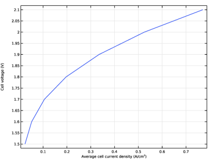
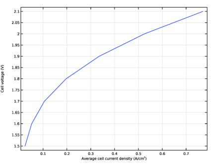
Select the x-axis label checkbox. In the associated text field, type Average cell current density (A/cm<sup>2</sup>).
|
|
6
|
|
1
|
|
2
|
|
1
|
|
2
|
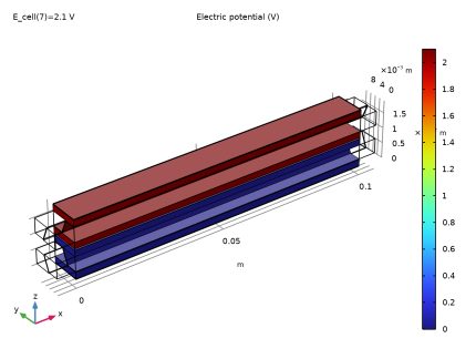
In the Settings window for Surface, click Replace Expression in the upper-right corner of the Expression section. From the menu, choose Component 1 (comp1) > Water Electrolyzer > we.phis - Electric potential - V.
|
|
3
|
|
1
|
|
2
|
|
1
|
|
2
|
|
3
|
|
1
|
|
2
|
|
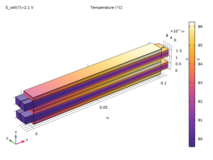
1
|
|
2
|
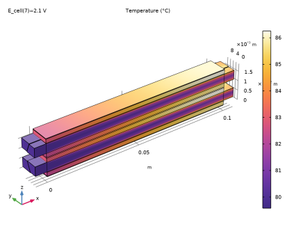
In the Settings window for Surface, click Replace Expression in the upper-right corner of the Expression section. From the menu, choose Component 1 (comp1) > Heat Transfer in Solids and Fluids > Temperature > T - Temperature - K.
|
|
3
|
|
4
|
|
5
|
|
1
|
|
2
|
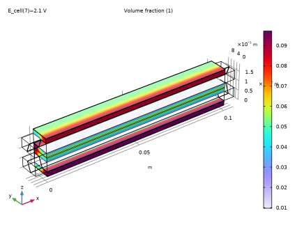
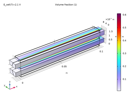
In the Settings window for 3D Plot Group, type Gas Volume Fraction in Channels in the Label text field.
|
|
3
|
|
4
|
|
1
|
|
2
|
In the Settings window for Volume, click Replace Expression in the upper-right corner of the Expression section. From the menu, choose Component 1 (comp1) > Phase Transport in Free and Porous Media Flow > s_g - Volume fraction - 1.
|
|
3
|
|
4
|
|
1
|
|
2
|
|
3
|
|
4
|
|
1
|
|
2
|
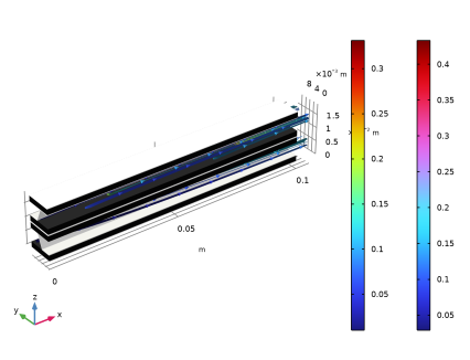
In the Settings window for 3D Plot Group, type Gas Volume Fractions and Streamlines in the Label text field.
|
|
3
|
|
4
|
|
1
|
|
2
|
In the Settings window for Streamline, click Replace Expression in the upper-right corner of the Expression section. From the menu, choose Component 1 (comp1) > Phase Transport in Free and Porous Media Flow > phtr.Nx_s_g,...,phtr.Nz_s_g - Mass flux, phase s_g.
|
|
3
|
|
4
|
|
5
|
Locate the Coloring and Style section. Find the Line style subsection. From the Type list, choose Ribbon.
|
|
6
|
|
1
|
|
2
|
In the Settings window for Color Expression, click Replace Expression in the upper-right corner of the Expression section. From the menu, choose Component 1 (comp1) > Phase Transport in Free and Porous Media Flow > s_g - Volume fraction - 1.
|
|
1
|
|
2
|
|
3
|
|
4
|
|
1
|
|
2
|
|
3
|
|
1
|
|
2
|
|
3
|
|
4
|
|
1
|
|
2
|
|
3
|
|
1
|
|
2
|
|
3
|
|
4
|
|
1
|
|
2
|
|
3
|
|
1
|
|
2
|
|
3
|
|
1
|
|
2
|
|
3
|
|
1
|
|
2
|
|
3
|
|
1
|
|
2
|
|
3
|
|
4
|
|
1
|
|
2
|
|
3
|
|
4
|
|
5
|
|
6
|
|
1
|
|
2
|
|
3
|
|
4
|
|
5
|