PDF

Ammonia-Fed Solid Oxide Fuel Cell
Introduction
In this model of an ammonia-fed solid oxide fuel cell (SOFC), the required hydrogen is supplied through endothermic thermal decomposition of ammonia. The model includes the full coupling between the mass balances and gas flow in the H2 and O2 gas-diffusion electrodes, the momentum balances in the H2 and O2 gas-flow channels, the energy balance across the cell, the balance of the ionic current carried by the oxide ion, and an electronic-current balance. A thermal decomposition reaction of ammonia is included in the H2 gas diffusion electrode domain.
The model computes the spatial distributions of the various species across the gas-diffusion electrodes and gas-flow channels. It demonstrates that the SOFC is cooled down at the lower applied current density and heated up at the higher applied current density.
The model also demonstrates the use of auxiliary species in the H2 gas mixture. The model is based on Ref. 1.
Model Definition
On the cathode, oxygen gas is reduced to form oxygen ions,
(1)
whereas on the anode, hydrogen gas is oxidized to form water vapor:
(2)
A thermal decomposition reaction of ammonia is included in the H2 gas-diffusion electrode domain:
(3)
Since the ammonia decomposition is an endothermic reaction, this reaction will absorb heat and cool down the SOFC. The cooling rate from decomposition will hence depend on the fuel flow rate into the cell.
Figure 1 shows the model geometry. Seven computational domains are used in the model: the two interconnects, H2 and O2 gas-flow channels, H2 and O2 gas-diffusion electrodes, and the membrane.
Figure 1: Model geometry. From top: Interconnect, O2 gas channel, O2 gas-diffusion electrode, solid oxide electrolyte layer, H2 gas-diffusion electrode, H2 gas-flow channel, and interconnect. The inlet and outlet positions are indicated in the figure.
The Hydrogen Fuel Cell interface is used to define the electrode reactions and the electrolyte charge transport in the porous gas-diffusion electrodes and the electrolyte layer, as well as the mass transport of the gas mixture. The current distribution is defined assuming a temperature-dependent electrolyte conductivity of the solid electrolyte.
The gas mixture at the anode consists of H2, H2O, N2, and NH3, whereas that at the cathode the mixture consists of O2 and N2. NH3 is added as an Auxiliary Species in the H2 gas mixture and its properties are set using the Thermodynamics node. The molar fraction initial values for the H2 gas mixture are derived assuming a close to 100% decomposition of NH3, since this reaction is so fast.
The composition of the gas mixture changes as a result of the electrochemical reactions and the thermal decomposition reaction of ammonia. On the anode side, the electrode kinetics depends on the local concentrations of H2O and H2 and on the cathode side, the electrode kinetics depends on the local concentrations of O2, according to the law of mass action (and the Nernst equation).
The mass transport of the gaseous species is modeled in the gas-flow channels and the gas-diffusion electrodes coupled to the resulting (laminar) flow of the gas mixture. The momentum flow is defined using the Free and Porous Media Flow, Brinkman interface for the H2 and O2 gas mixtures separately in the gas-flow channels and the gas-diffusion electrodes.
The properties of the gas mixtures at both anode and cathode, as well as the equilibrium potentials of the electrode reactions, are automatically defined by the default built-in options of the Hydrogen Fuel Cell interface.
For average cell currents above 0.1 A/cm2, the molar flow rates of ammonia and oxygen are set to be proportional to the total current, with a 25% excess of ammonia and a 300% excess of oxygen (that is, using ammonia and oxygen flow stoichiometries of 1.25 and 4, respectively). Below 0.1 A/cm2 the flow rates are held constant, corresponding to the flow rates values for a 1.25/4 stoichiometry at 0.1 A/cm2.
The model is solved using an Auxiliary sweep, ramping up the average cell current density from 0.01 to 1 A/cm2.
Results and Discussion
Figure 2 shows the change in the cell voltage and outlet temperature for different applied current densities. It can be seen in Figure 2 that the cell voltage decreases and the cell outlet temperature increases with an increase in the applied current density. The cell is cooled down for an applied current density of up to 0.1 A/cm2, which is attributed to constant thermal decomposition of NH3. Since the fuel stoichiometry for the flow rate is higher than 1.25/4 at currents below 0.1 A/cm2, the decomposition reaction will cool the cell relatively more for low currents. In addition, the lower overpotentials at lower currents will generate relatively less heat for lower currents. The increase in the cell temperature beyond applied current density of 0.1 A/cm2 is attributed to the increased cell heating due to the increased voltage losses.
Figure 2: Change in cell voltage and outlet temperature at different applied current densities.
Figure 3 shows the change in temperature across the SOFC cell for applied current densities of 0.01 A/cm2 (left) and 1 A/cm2 (right). The negative change in temperature indicates that the cell is cooled down at an applied current density of 0.01 A/cm2, whereas the positive change in temperature indicates that the cell is heated up at an applied current density of 1 A/cm2.
Figure 3: Change in temperature at applied current density 0.01 A/cm2 (left) and 1 A/cm2(right).
Figure 4 shows the change in thermal decomposition reaction rate of ammonia across the SOFC cell for applied current densities of 0.01 A/cm2 (left) and 1 A/cm2 (right). The ammonia thermal decomposition rate increases with an increase in the applied current density, which is attributed to the increased cell temperature.
Figure 4: Change in thermal decomposition reaction rate of ammonia at applied current density 0.01 A/cm2 (left) and 1 A/cm2 (right).
Figure 5 shows the change in ammonia concentration across the SOFC cell for applied current densities of 0.01 A/cm2 (left) and 1 A/cm2 (right). The ammonia concentration is more uniform at 0.01 A/cm2 as compared to 1 A/cm2, which is attributed to the higher ammonia thermal decomposition rate at the higher applied current density.
Figure 5: Change in ammonia concentration at applied current density 0.01 A/cm2 (left) and 1 A/cm2 (right).
Reference
1. M. Ni, “Thermo-electrochemical modeling of ammonia-fueled solid oxide fuel cells considering ammonia thermal decomposition in the anode,” Int. J. Hydrog. Energy, vol. 36, p. 3153, 2011.
Application Library path: Fuel_Cell_and_Electrolyzer_Module/Fuel_Cells/sofc_nh3
Modeling Instructions
From the File menu, choose New.
New
In the New window, click  Model Wizard.
Model Wizard
1
In the Model Wizard window, click  2D.
2
In the Select Physics tree, select Electrochemistry > Hydrogen Fuel Cells > Solid Oxide (fc).
3
Click Add.
4
In the Select Physics tree, select Fluid Flow > Porous Media and Subsurface Flow > Free and Porous Media Flow, Brinkman (fp).
5
Click Add.
6
In the Velocity field (m/s) text field, type ua.
7
In the Velocity field components table, enter the following settings:
8
In the Pressure (Pa) text field, type pa.
9
Click Add.
10
In the Velocity field (m/s) text field, type uc.
11
In the Velocity field components table, enter the following settings:
12
In the Pressure (Pa) text field, type pc.
13
In the Select Physics tree, select Heat Transfer > Heat Transfer in Solids and Fluids (ht).
14
Click Add.
15
Click  Study.
16
In the Select Study tree, select Preset Studies for Selected Physics Interfaces > Hydrogen Fuel Cell > Stationary with Initialization.
17
Global Definitions
Parameters 1
First load the model parameters.
1
In the Model Builder window, under Global Definitions click Parameters 1.
2
In the Settings window for Parameters, locate the Parameters section.
3
Click  Load from File.
4
Geometry 1
Draw the model geometry using a rectangle and six layers and two inlets for extended inlets.
1
In the Sketch toolbar, click Rectangle and choose Rectangle.
Rectangle 1 (r1)
1
In the Model Builder window, expand the Geometry 1 node.
2
Right-click Component 1 (comp1) > Geometry 1 and choose Rectangle.
3
In the Settings window for Rectangle, locate the Size and Shape section.
4
In the Width text field, type L.
5
In the Height text field, type W.
6
Click to expand the Layers section. In the table, enter the following settings:
7
In the Sketch toolbar, click Rectangle and choose Rectangle.
Rectangle 2 (r2)
1
In the Geometry toolbar, click  Rectangle.
2
In the Settings window for Rectangle, locate the Size and Shape section.
3
In the Width text field, type din.
4
In the Height text field, type dg.
5
Locate the Position section. In the x text field, type -din.
6
In the y text field, type di.
7
In the Sketch toolbar, click Rectangle and choose Rectangle.
Rectangle 3 (r3)
1
In the Geometry toolbar, click  Rectangle.
2
In the Settings window for Rectangle, locate the Size and Shape section.
3
In the Width text field, type din.
4
In the Height text field, type dg.
5
Locate the Position section. In the x text field, type -din.
6
In the y text field, type di+dg+da+dm+dc.
7
Click  Build All Objects.
8
Click the  Zoom Extents button in the Graphics toolbar.
Definitions
Variables 1
Next, add variables.
1
In the Definitions toolbar, click  Local Variables.
2
In the Settings window for Variables, locate the Variables section.
3
Click  Load from File.
4
Global Definitions
Add thermodynamic properties for ammonia.
1
In the Physics toolbar, click  Thermodynamics and choose Thermodynamic System.
Select System
1
Go to the Select System window.
2
Click the Next button in the window toolbar.
Select Species
1
Go to the Select Species window.
2
In the Species list box, select ammonia (7664-41-7, H3N).
3
Click  Add Selected.
4
Click the Next button in the window toolbar.
Select Thermodynamic Model
1
Go to the Select Thermodynamic Model window.
2
Click the Finish button in the window toolbar.
Global Definitions
Gas System 1 (pp1)
Right-click Global Definitions > Thermodynamics > Gas System 1 (pp1) and choose Species Property.
Select Properties
1
Go to the Select Properties window.
2
In the list, choose Enthalpy of formation (J/mol), Entropy of formation (J/(K*mol)), Fuller diffusion volume (cm^3), Heat capacity (Cp) (J/(K*mol)), Molar mass (g/mol), Normal boiling-point temperature (K), Thermal conductivity (W/(m*K)), and Viscosity (Pa*s).
3
Click  Add Selected.
4
Click the Next button in the window toolbar.
Select Phase
1
Go to the Select Phase window.
2
Click the Next button in the window toolbar.
Select Species
1
Go to the Select Species window.
2
3
Click  Add Selected.
4
Click the Next button in the window toolbar.
Species Property Overview
1
Go to the Species Property Overview window.
2
Click the Finish button in the window toolbar.
Hydrogen Fuel Cell (fc)
Start setting up the electrochemistry part of the model.
1
In the Model Builder window, under Component 1 (comp1) click Hydrogen Fuel Cell (fc).
2
In the Settings window for Hydrogen Fuel Cell, locate the Domain Selection section.
3
4
Click  Remove from Selection.
5
6
7
Click  Remove from Selection.
8
9
Locate the H2 Gas Mixture section. Select the N2 checkbox.
10
Select the Auxiliary species checkbox.
11
Click to expand the Electrode Reaction Settings section. Find the Built-in thermodynamic expressions subsection. In the TRHE text field, type T_in.
12
Locate the Out-of-Plane Thickness section. In the dz text field, type D.
Membrane 1
1
In the Physics toolbar, click  Domains and choose Membrane.
2
H2 Gas Diffusion Electrode 1
1
In the Physics toolbar, click  Domains and choose H2 Gas Diffusion Electrode.
2
3
In the Settings window for H2 Gas Diffusion Electrode, locate the Effective Electrolyte Charge Transport section.
4
In the εl text field, type epsl.
5
Locate the Gas Transport section. From the Effective diffusivity correction list, choose Tortuosity.
6
In the εg text field, type epsg.
7
In the τg text field, type taug.
8
Select the Include pore-wall interaction checkbox.
9
In the dpore text field, type d_pore.
H2 Gas Diffusion Electrode Reaction 1
1
In the Model Builder window, click H2 Gas Diffusion Electrode Reaction 1.
2
In the Settings window for H2 Gas Diffusion Electrode Reaction, locate the Electrode Kinetics section.
3
In the i0,ref(T) text field, type i0_ref_H2.
4
Locate the Active Specific Surface Area section. In the av text field, type S.
O2 Gas Diffusion Electrode 1
1
In the Physics toolbar, click  Domains and choose O2 Gas Diffusion Electrode.
2
3
In the Settings window for O2 Gas Diffusion Electrode, locate the Effective Electrolyte Charge Transport section.
4
In the εl text field, type epsl.
5
Locate the Gas Transport section. From the Effective diffusivity correction list, choose Tortuosity.
6
In the εg text field, type epsg.
7
In the τg text field, type taug.
8
Select the Include pore-wall interaction checkbox.
9
In the dpore text field, type d_pore.
O2 Gas Diffusion Electrode Reaction 1
1
In the Model Builder window, click O2 Gas Diffusion Electrode Reaction 1.
2
In the Settings window for O2 Gas Diffusion Electrode Reaction, locate the Electrode Kinetics section.
3
In the i0,ref(T) text field, type i0_ref_O2.
4
In the αa text field, type 0.5.
5
Locate the Active Specific Surface Area section. In the av text field, type S.
H2 Gas Flow Channel 1
Next, add the H2 Gas Flow Channel.
1
In the Physics toolbar, click  Domains and choose H2 Gas Flow Channel.
2
O2 Gas Flow Channel 1
Next, add the O2 Gas Flow Channel.
1
In the Physics toolbar, click  Domains and choose O2 Gas Flow Channel.
2
Electronic Conducting Phase 1
Next, specify the initial values for the oxygen domain to enhance convergence and set the boundary conditions.
1
In the Model Builder window, click Electronic Conducting Phase 1.
Initial Values, O2 Domains 1
1
In the Physics toolbar, click  Attributes and choose Initial Values, O2 Domains.
2
Electronic Conducting Phase 1
In the Model Builder window, click Electronic Conducting Phase 1.
Electric Ground 1
1
In the Physics toolbar, click  Attributes and choose Electric Ground.
2
Electronic Conducting Phase 1
In the Model Builder window, click Electronic Conducting Phase 1.
Electrode Current 1
1
In the Physics toolbar, click  Attributes and choose Electrode Current.
2
3
In the Settings window for Electrode Current, locate the Electrode Current section.
4
In the Is,total text field, type -I_tot.
H2 Gas Phase 1
Set dynamic viscosity to built in and set thermodynamics properties for auxiliary species.
1
In the Model Builder window, under Component 1 (comp1) > Hydrogen Fuel Cell (fc) click H2 Gas Phase 1.
2
In the Settings window for H2 Gas Phase, locate the Auxiliary Species section.
3
In the Maux text field, type M_aux.
4
In the Haux(T) text field, type H_aux.
5
In the Saux(T) text field, type S_aux.
6
In the Cp,aux(T) text field, type Cp_aux.
7
In the νaux text field, type nu_aux.
8
In the μaux text field, type mu_aux.
9
In the kaux text field, type k_aux.
10
In the Tb,aux text field, type Tb_aux.
Next, specify initial values, add the ammonia decomposition reaction, and set the hydrogen inlet and outlet boundary conditions.
Initial Values 1
1
In the Model Builder window, click Initial Values 1.
2
In the Settings window for Initial Values, locate the Initial Composition section.
3
In the x0,H2O text field, type x0_H2O_an.
4
In the x0,N2 text field, type x0_N2_an.
5
In the x0,aux text field, type x0_NH3_an.
H2 Gas Phase 1
1
Click the  Show More Options button in the Model Builder toolbar.
2
In the Show More Options dialog, select Physics > Advanced Physics Options in the tree.
3
In the tree, select the checkbox for the node Physics > Advanced Physics Options.
4
5
In the Model Builder window, click H2 Gas Phase 1.
Reaction Sources 1
1
In the Physics toolbar, click  Attributes and choose Reaction Sources.
2
3
In the Settings window for Reaction Sources, locate the Reaction Sources section.
4
From the Source type list, choose Molar.
5
In the rH2 text field, type 1.5*r_NH3.
6
In the rN2 text field, type 0.5*r_NH3.
7
In the raux text field, type -r_NH3.
H2 Gas Phase 1
In the Model Builder window, click H2 Gas Phase 1.
H2 Inlet 1
1
In the Physics toolbar, click  Attributes and choose H2 Inlet.
2
3
In the Settings window for H2 Inlet, locate the Inlet Flow Type section.
4
Clear the Stoichiometric feed checkbox.
5
Locate the Mass Flow Rates section. In the J0,aux text field, type m_NH3_an.
6
Locate the Boundary Initial Values section. From the list, choose User defined.
7
In the ω0,bnd,H2O text field, type w0_H2O_an.
8
In the ω0,bnd,N2 text field, type w0_N2_an.
9
In the ω0,bnd,aux text field, type w0_NH3_an.
H2 Gas Phase 1
In the Model Builder window, click H2 Gas Phase 1.
H2 Outlet 1
1
In the Physics toolbar, click  Attributes and choose H2 Outlet.
2
O2 Gas Phase 1
Next, set the initial values and the oxygen inlet and outlet boundary conditions.
Initial Values 1
1
In the Model Builder window, expand the O2 Gas Phase 1 node, then click Initial Values 1.
2
In the Settings window for Initial Values, locate the Initial Composition section.
3
In the x0,N2 text field, type x0_N2_cath.
O2 Gas Phase 1
In the Model Builder window, click O2 Gas Phase 1.
O2 Inlet 1
1
In the Physics toolbar, click  Attributes and choose O2 Inlet.
2
3
In the Settings window for O2 Inlet, locate the Stoichiometric Feed section.
4
In the I text field, type I_flow.
5
In the SO2 text field, type stoich_O2.
O2 Gas Phase 1
In the Model Builder window, click O2 Gas Phase 1.
O2 Outlet 1
1
In the Physics toolbar, click  Attributes and choose O2 Outlet.
2
Free and Porous Media Flow, Brinkman - H2 side
Next set flow physics at H2 and O2 sides separately.
1
In the Model Builder window, under Component 1 (comp1) click Free and Porous Media Flow, Brinkman (fp).
2
In the Settings window for Free and Porous Media Flow, Brinkman, type Free and Porous Media Flow, Brinkman - H2 side in the Label text field.
3
Locate the Domain Selection section. Click  Clear Selection.
4
5
Locate the Physical Model section. From the Compressibility list, choose Compressible flow (Ma<0.3).
Porous Medium 1
1
In the Physics toolbar, click  Domains and choose Porous Medium.
2
Porous Matrix 1
1
In the Model Builder window, click Porous Matrix 1.
2
In the Settings window for Porous Matrix, locate the Matrix Properties section.
3
From the εp list, choose User defined. In the associated text field, type epsg.
4
From the κ list, choose User defined. In the associated text field, type kappag_GDE.
Inlet 1
1
In the Physics toolbar, click  Boundaries and choose Inlet.
2
3
In the Settings window for Inlet, locate the Boundary Condition section.
4
5
Locate the Mass Flow section. In the m text field, type m_NH3_an.
Outlet 1
1
In the Physics toolbar, click  Boundaries and choose Outlet.
2
Free and Porous Media Flow, Brinkman - O2 Side
1
In the Model Builder window, under Component 1 (comp1) click Free and Porous Media Flow, Brinkman 2 (fp2).
2
In the Settings window for Free and Porous Media Flow, Brinkman, type Free and Porous Media Flow, Brinkman - O2 Side in the Label text field.
3
Locate the Domain Selection section. Click  Clear Selection.
4
5
Locate the Physical Model section. From the Compressibility list, choose Compressible flow (Ma<0.3).
Porous Medium 1
1
In the Physics toolbar, click  Domains and choose Porous Medium.
2
Porous Matrix 1
1
In the Model Builder window, click Porous Matrix 1.
2
In the Settings window for Porous Matrix, locate the Matrix Properties section.
3
From the εp list, choose User defined. In the associated text field, type epsg.
4
From the κ list, choose User defined. In the associated text field, type kappag_GDE.
Inlet 1
1
In the Physics toolbar, click  Boundaries and choose Inlet.
2
3
In the Settings window for Inlet, locate the Boundary Condition section.
4
5
Locate the Mass Flow section. In the m text field, type fc.o2gasph1.o2in1.J0.
Outlet 1
1
In the Physics toolbar, click  Boundaries and choose Outlet.
2
Heat Transfer in Solids and Fluids (ht)
Next, set the heat transfer physics.
1
In the Model Builder window, under Component 1 (comp1) click Heat Transfer in Solids and Fluids (ht).
2
In the Settings window for Heat Transfer in Solids and Fluids, locate the Physical Model section.
3
In the Tref text field, type T_in.
Solid: Interconnects
1
In the Model Builder window, under Component 1 (comp1) > Heat Transfer in Solids and Fluids (ht) click Solid 1.
2
In the Settings window for Solid, type Solid: Interconnects in the Label text field.
Fluid: Flow Channels
1
In the Model Builder window, under Component 1 (comp1) > Heat Transfer in Solids and Fluids (ht) click Fluid 1.
2
In the Settings window for Fluid, type Fluid: Flow Channels in the Label text field.
3
4
Locate the Heat Conduction, Fluid section. From the k list, choose Thermal conductivity, gas phase (fc).
5
Locate the Thermodynamics, Fluid section. From the Fluid type list, choose Gas/Liquid.
6
From the ρ list, choose Density of gas phase (fc).
7
From the Cp list, choose Heat capacity at constant pressure, gas phase (fc).
Initial Values 1
1
In the Model Builder window, click Initial Values 1.
2
In the Settings window for Initial Values, locate the Initial Values section.
3
In the T text field, type T_in.
Porous Medium: Anode GDE
Next, add thermal conductivity, density and heat capacity for the gas diffusion electrode domains.
1
In the Physics toolbar, click  Domains and choose Porous Medium.
2
In the Settings window for Porous Medium, type Porous Medium: Anode GDE in the Label text field.
3
Fluid 1
1
In the Model Builder window, click Fluid 1.
2
In the Settings window for Fluid, locate the Heat Conduction, Fluid section.
3
From the kf list, choose Thermal conductivity, gas phase (fc).
4
Locate the Thermodynamics, Fluid section. From the ρf list, choose Density of gas phase (fc).
5
From the Cp,f list, choose Heat capacity at constant pressure, gas phase (fc).
Porous Matrix 1
1
In the Model Builder window, click Porous Matrix 1.
2
In the Settings window for Porous Matrix, locate the Matrix Properties section.
3
From the εp list, choose User defined. In the associated text field, type epsg.
4
Locate the Heat Conduction, Porous Matrix section. From the kb list, choose User defined. In the associated text field, type ka.
5
Locate the Thermodynamics, Porous Matrix section. From the ρb list, choose User defined. From the Cp,b list, choose User defined.
Porous Medium: Cathode GDE
1
In the Physics toolbar, click  Domains and choose Porous Medium.
2
In the Settings window for Porous Medium, type Porous Medium: Cathode GDE in the Label text field.
3
Fluid 1
1
In the Model Builder window, click Fluid 1.
2
In the Settings window for Fluid, locate the Heat Conduction, Fluid section.
3
From the kf list, choose Thermal conductivity, gas phase (fc).
4
Locate the Thermodynamics, Fluid section. From the ρf list, choose Density of gas phase (fc).
5
From the Cp,f list, choose Heat capacity at constant pressure, gas phase (fc).
Porous Matrix 1
1
In the Model Builder window, click Porous Matrix 1.
2
In the Settings window for Porous Matrix, locate the Matrix Properties section.
3
From the εp list, choose User defined. In the associated text field, type epsg.
4
Locate the Heat Conduction, Porous Matrix section. From the kb list, choose User defined. In the associated text field, type kc.
5
Locate the Thermodynamics, Porous Matrix section. From the ρb list, choose User defined. From the Cp,b list, choose User defined.
Solid: Membrane
Next, add thermal conductivity for the membrane domains.
1
In the Physics toolbar, click  Domains and choose Solid.
2
In the Settings window for Solid, type Solid: Membrane in the Label text field.
3
4
Locate the Heat Conduction, Solid section. From the k list, choose User defined. In the associated text field, type km.
5
Locate the Thermodynamics, Solid section. From the ρ list, choose User defined. From the Cp list, choose User defined.
Inflow 1
Next, add the inflow, outflow, and periodic condition boundary conditions.
1
In the Physics toolbar, click  Boundaries and choose Inflow.
2
3
In the Settings window for Inflow, locate the Upstream Properties section.
4
In the Tustr text field, type T_in.
Outflow 1
1
In the Physics toolbar, click  Boundaries and choose Outflow.
2
Periodic Condition 1
1
In the Physics toolbar, click  Boundaries and choose Periodic Condition.
2
Multiphysics
Next, add a few multiphysics coupling nodes for electrochemical heating, nonisothermal flow and reacting flow.
Electrochemical Heating 1 (ech1)
In the Physics toolbar, click  Multiphysics Couplings and choose Domain > Electrochemical Heating.
Nonisothermal Flow 1 (nitf1)
In the Physics toolbar, click  Multiphysics Couplings and choose Domain > Nonisothermal Flow.
Nonisothermal Flow 2 (nitf2)
1
In the Physics toolbar, click  Multiphysics Couplings and choose Domain > Nonisothermal Flow.
2
In the Settings window for Nonisothermal Flow, locate the Coupled Interfaces section.
3
From the Fluid flow list, choose Free and Porous Media Flow, Brinkman - O2 Side (fp2).
Reacting Flow, H2 Gas Phase 1 (rfh1)
In the Physics toolbar, click  Multiphysics Couplings and choose Domain > Reacting Flow, H2 Gas Phase.
Reacting Flow, O2 Gas Phase 1 (rfo1)
1
In the Physics toolbar, click  Multiphysics Couplings and choose Domain > Reacting Flow, O2 Gas Phase.
2
In the Settings window for Reacting Flow, O2 Gas Phase, locate the Coupled Interfaces section.
3
From the Fluid flow list, choose Free and Porous Media Flow, Brinkman - O2 Side (fp2).
Definitions
Next, add a couple of probes to be used later in postprocessing.
Global Variable Probe 1 (var1)
1
In the Definitions toolbar, click  Probes and choose Global Variable Probe.
2
In the Settings window for Global Variable Probe, locate the Expression section.
3
In the Expression text field, type fc.phis0_ec1.
4
Click to expand the Table and Window Settings section. From the Output table list, choose New table.
5
Click  Add Plot Window.
Point Probe 1 (point1)
1
In the Definitions toolbar, click  Probes and choose Point Probe.
2
In the Settings window for Point Probe, locate the Source Selection section.
3
Click  Clear Selection.
4
5
Locate the Expression section. In the Expression text field, type T.
6
Click to expand the Table and Window Settings section. From the Output table list, choose New table.
7
From the Plot window list, choose Probe Plot 1.
Materials
Now, add materials from the Material Library.
Add Material
1
In the Home toolbar, click  Add Material to open the Add Material window.
2
Go to the Add Material window.
3
In the tree, select Fuel Cell and Electrolyzer > Solid Oxides > Yttria-Stabilized Zirconia, 8YSZ, (ZrO2)0.92-(Y2O3)0.08.
4
Click the Add to Component button in the window toolbar.
Materials
Yttria-Stabilized Zirconia, 8YSZ, (ZrO2)0.92-(Y2O3)0.08 (mat1)
1
In the Settings window for Material, locate the Geometric Entity Selection section.
2
Click  Clear Selection.
3
Add Material
1
Go to the Add Material window.
2
In the tree, select Built-in > Steel AISI 4340.
3
Click the Add to Component button in the window toolbar.
4
In the Materials toolbar, click  Add Material to close the Add Material window.
Materials
Steel AISI 4340 (mat2)
Select Domains 3 and 9 only.
Mesh 1
Next, set up a user-controlled mesh.
Distribution 1
1
In the Model Builder window, under Component 1 (comp1) right-click Mesh 1 and choose Distribution.
2
3
In the Settings window for Distribution, locate the Distribution section.
4
From the Distribution type list, choose Predefined.
5
In the Number of elements text field, type 100.
6
In the Element ratio text field, type 10.
7
Select the Reverse direction checkbox.
Distribution 2
1
In the Model Builder window, right-click Mesh 1 and choose Distribution.
2
3
In the Settings window for Distribution, locate the Distribution section.
4
In the Number of elements text field, type 2.
Distribution 3
1
Right-click Mesh 1 and choose Distribution.
2
3
In the Settings window for Distribution, locate the Distribution section.
4
From the Distribution type list, choose Predefined.
5
In the Number of elements text field, type 10.
6
In the Element ratio text field, type 2.
7
Select the Symmetric distribution checkbox.
Distribution 4
1
Right-click Mesh 1 and choose Distribution.
2
3
In the Settings window for Distribution, locate the Distribution section.
4
In the Number of elements text field, type 2.
Distribution 5
1
Right-click Mesh 1 and choose Distribution.
2
3
In the Settings window for Distribution, locate the Distribution section.
4
From the Distribution type list, choose Predefined.
5
In the Number of elements text field, type 40.
6
In the Element ratio text field, type 10.
7
From the Growth rate list, choose Exponential.
Distribution 6
1
Right-click Mesh 1 and choose Distribution.
2
3
In the Settings window for Distribution, locate the Distribution section.
4
From the Distribution type list, choose Predefined.
5
In the Number of elements text field, type 40.
6
In the Element ratio text field, type 10.
7
From the Growth rate list, choose Exponential.
8
Select the Symmetric distribution checkbox.
Distribution 7
1
Right-click Mesh 1 and choose Distribution.
2
3
In the Settings window for Distribution, locate the Distribution section.
4
In the Number of elements text field, type 20.
Mapped 1
1
In the Mesh toolbar, click  Mapped.
2
In the Settings window for Mapped, click  Build All.
3
Click the  Zoom Extents button in the Graphics toolbar.
The mesh should look like this:
Study 1
Finally, set the current distribution initialization, flow initialization, and stationary study settings using an auxiliary sweep for the average cell current density to complete the model setup.
Step 3: Stationary 2
In the Study toolbar, click  Stationary.
Step 1: Current Distribution Initialization
1
In the Model Builder window, click Step 1: Current Distribution Initialization.
2
In the Settings window for Current Distribution Initialization, locate the Study Settings section.
3
From the Current distribution type list, choose Secondary.
Stationary - Flow Initialization
1
In the Model Builder window, click Step 2: Stationary.
2
In the Settings window for Stationary, type Stationary - Flow Initialization in the Label text field.
3
Locate the Physics and Variables Selection section. In the Solve for column of the table, under Component 1 (comp1), clear the checkboxes for Hydrogen Fuel Cell (fc) and Heat Transfer in Solids and Fluids (ht).
4
In the Solve for column of the table, under Component 1 (comp1) > Multiphysics, clear the checkboxes for Electrochemical Heating 1 (ech1), Nonisothermal Flow 1 (nitf1), and Nonisothermal Flow 2 (nitf2).
Stationary - All Physics
1
In the Model Builder window, under Study 1 click Step 3: Stationary 2.
2
In the Settings window for Stationary, type Stationary - All Physics in the Label text field.
3
Click to expand the Study Extensions section. Select the Auxiliary sweep checkbox.
4
5
Solution 1 (sol1)
1
In the Study toolbar, click  Show Default Solver.
2
In the Model Builder window, expand the Solution 1 (sol1) node.
3
In the Model Builder window, expand the Study 1 > Solver Configurations > Solution 1 (sol1) > Stationary Solver 3 node.
4
Right-click Study 1 > Solver Configurations > Solution 1 (sol1) > Stationary Solver 3 and choose Fully Coupled.
5
In the Settings window for Fully Coupled, click to expand the Method and Termination section.
6
In the Maximum number of iterations text field, type 100.
7
From the Termination criterion list, choose Solution.
8
In the Study toolbar, click  Compute.
Results
Some plots are added by default. Follow the instructions below to reproduce the figures in the Results and Discussion section.
Voltage and Temperature
1
In the Model Builder window, expand the Results > Probe Plot Group 1 node, then click Probe Plot Group 1.
2
In the Settings window for 1D Plot Group, type Voltage and Temperature in the Label text field.
3
Locate the Plot Settings section.
4
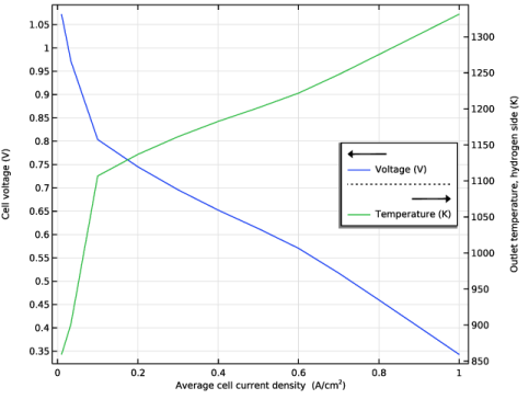
Select the x-axis label checkbox. In the associated text field, type Average cell current density (A/cm<sup>2</sup>).
5
Select the Two y-axes checkbox.
6
Select the y-axis label checkbox. In the associated text field, type Cell voltage (V).
7
Select the Secondary y-axis label checkbox. In the associated text field, type Outlet temperature, hydrogen side (K).
8
9
Locate the Legend section. From the Position list, choose Middle right.
Probe Table Graph 1
1
In the Model Builder window, click Probe Table Graph 1.
2
In the Settings window for Table Graph, click to expand the Legends section.
3
From the Legends list, choose Manual.
4
Probe Table Graph 2
1
In the Model Builder window, click Probe Table Graph 2.
2
In the Settings window for Table Graph, locate the Legends section.
3
From the Legends list, choose Manual.
4
Voltage and Temperature
1
In the Model Builder window, click Voltage and Temperature.
2
In the Voltage and Temperature toolbar, click  Plot.
The plot should look like Figure 2.
Surface 1
1
In the Model Builder window, expand the Temperature (ht) node, then click Surface 1.
2
In the Settings window for Surface, locate the Expression section.
3
In the Expression text field, type T-T_in.
Temperature (ht)
1
In the Model Builder window, click Temperature (ht).
2
In the Settings window for 2D Plot Group, click to expand the Title section.
3
From the Title type list, choose Manual.
4
In the Title text area, type Surface: Change in Temperature (K).
5
In the Parameter indicator text field, type I_avg=eval(I_avg,A/cm^2) A/cm<sup>2</sup>.
6
In the Temperature (ht) toolbar, click  Plot.
7
Locate the Data section. From the Parameter value (I_avg (A/cm^2)) list, choose 0.01.
8
In the Temperature (ht) toolbar, click  Plot.
The plots should look like Figure 3.
Ammonia Decomposition Reaction Rate
Next, plot ammonia thermal decomposition reaction rate over the hydrogen gas diffusion electrode and flow channel domains.
1
In the Results toolbar, click  2D Plot Group.
2
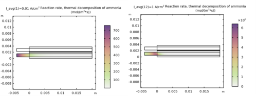
In the Settings window for 2D Plot Group, type Ammonia Decomposition Reaction Rate in the Label text field.
Surface 1
1
In the Ammonia Decomposition Reaction Rate toolbar, click  Surface.
2
In the Settings window for Surface, locate the Expression section.
3
In the Expression text field, type r_NH3.
4
Locate the Coloring and Style section. From the Color table list, choose HelfrichiZero.
Ammonia Decomposition Reaction Rate
1
In the Model Builder window, click Ammonia Decomposition Reaction Rate.
2
In the Ammonia Decomposition Reaction Rate toolbar, click  Plot.
3
In the Settings window for 2D Plot Group, locate the Data section.
4
From the Parameter value (I_avg (A/cm^2)) list, choose 0.01.
5
In the Ammonia Decomposition Reaction Rate toolbar, click  Plot.
The plots should look like Figure 4.
Surface 1
1
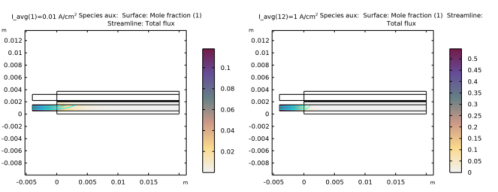
In the Model Builder window, expand the Results > Mole Fraction, aux (fc) node, then click Surface 1.
2
In the Settings window for Surface, locate the Coloring and Style section.
3
From the Color table list, choose ConopiformisZero.
Streamline 1
1
In the Model Builder window, expand the Results > Mole Fraction, aux (fc) node, then click Streamline 1.
2
In the Settings window for Streamline, locate the Streamline Positioning section.
3
From the Positioning list, choose Magnitude controlled.
4
In the Maximum density level text field, type 10.
5
Locate the Coloring and Style section. Find the Point style subsection.
6
Select the Scale factor checkbox. In the associated text field, type 0.06.
7
From the Color list, choose Cyan.
The plots should look like Figure 5.
8
In the Mole Fraction, aux (fc) toolbar, click  Plot.
Mole Fraction, aux (fc)
1
In the Model Builder window, click Mole Fraction, aux (fc).
2
In the Settings window for 2D Plot Group, locate the Data section.
3
From the Parameter value (I_avg (A/cm^2)) list, choose 0.01.
Streamline 1
1
In the Model Builder window, click Streamline 1.
2
In the Settings window for Streamline, locate the Streamline Positioning section.
3
From the Positioning list, choose Magnitude controlled.
4
In the Maximum density level text field, type 8.8.
5
Locate the Coloring and Style section. Find the Point style subsection. In the Scale factor text field, type 0.6.
6
In the Mole Fraction, aux (fc) toolbar, click  Plot.
Follow the instructions below to improve the appearance of the remaining plots.
Surface 1
1
In the Model Builder window, expand the Electrode Potential with Respect to Ground (fc) node, then click Surface 1.
2
In the Settings window for Surface, locate the Coloring and Style section.
3
From the Color table list, choose MetasepiaBlue.
Arrow Surface 1
1
In the Model Builder window, click Arrow Surface 1.
2
In the Settings window for Arrow Surface, locate the Coloring and Style section.
3
From the Color list, choose Yellow.
Surface 1
1
In the Model Builder window, expand the Results > Mole Fraction, H2 (fc) node, then click Surface 1.
2
In the Settings window for Surface, locate the Coloring and Style section.
3
From the Color table list, choose ConopiformisZero.
Streamline 1
1
In the Model Builder window, click Streamline 1.
2
In the Settings window for Streamline, locate the Streamline Positioning section.
3
From the Positioning list, choose Magnitude controlled.
4
In the Maximum density level text field, type 12.
5
Locate the Coloring and Style section. Find the Point style subsection. From the Color list, choose Cyan.
Surface 1
1
In the Model Builder window, expand the Results > Mole Fraction, O2 (fc) node, then click Surface 1.
2
In the Settings window for Surface, locate the Coloring and Style section.
3
From the Color table list, choose ConopiformisZero.
Streamline 1
1
In the Model Builder window, click Streamline 1.
2
In the Settings window for Streamline, locate the Streamline Positioning section.
3
From the Positioning list, choose Magnitude controlled.
4
In the Maximum density level text field, type 10.
5
Locate the Coloring and Style section. Find the Point style subsection. From the Color list, choose Cyan.
Surface 1
1
In the Model Builder window, expand the Results > Mole Fraction, H2O (fc) node, then click Surface 1.
2
In the Settings window for Surface, locate the Coloring and Style section.
3
From the Color table list, choose ConopiformisZero.
Streamline 1
1
In the Model Builder window, click Streamline 1.
2
In the Settings window for Streamline, locate the Streamline Positioning section.
3
From the Positioning list, choose Magnitude controlled.
4
In the Maximum density level text field, type 10.
5
Locate the Coloring and Style section. Find the Point style subsection. From the Color list, choose Cyan.
Surface 1
1
In the Model Builder window, expand the Results > Mole Fraction, N2 (fc) node, then click Surface 1.
2
In the Settings window for Surface, locate the Coloring and Style section.
3
From the Color table list, choose ConopiformisZero.
Streamline 1
1
In the Model Builder window, click Streamline 1.
2
In the Settings window for Streamline, locate the Streamline Positioning section.
3
From the Positioning list, choose Magnitude controlled.
4
In the Maximum density level text field, type 10.
5
Locate the Coloring and Style section. Find the Point style subsection. From the Color list, choose Cyan.