|
|
|
|
1
|
|
2
|
In the Select Physics tree, select Electrochemistry > Primary and Secondary Current Distribution > Secondary Current Distribution (cd).
|
|
3
|
Click Add.
|
|
4
|
Click
|
|
5
|
In the Select Study tree, select Preset Studies for Selected Physics Interfaces > Stationary with Initialization.
|
|
6
|
Click
|
|
1
|
|
2
|
Browse to the model’s Application Libraries folder and double-click the file soec_thermodynamics_geom_sequence.mph.
|
|
3
|
|
4
|
|
1
|
|
2
|
|
1
|
|
2
|
|
3
|
|
4
|
Browse to the model’s Application Libraries folder and double-click the file soec_thermodynamics_physics_parameters.txt.
|
|
5
|
|
1
|
Go to the Select System window.
|
|
2
|
Click the Next button in the window toolbar.
|
|
1
|
Go to the Select Species window.
|
|
2
|
|
3
|
Click
|
|
4
|
|
5
|
Click
|
|
6
|
Click the Next button in the window toolbar.
|
|
1
|
Go to the Select Thermodynamic Model window.
|
|
2
|
Click the Finish button in the window toolbar.
|
|
1
|
In the Settings window for Thermodynamic System, type Gas System - H2 and H2O in the Label text field.
|
|
2
|
Right-click Global Definitions > Thermodynamics > Gas System - H2 and H2O and choose Generate Chemistry.
|
|
1
|
Go to the Select Species window.
|
|
2
|
|
3
|
Click
|
|
4
|
Click the Next button in the window toolbar.
|
|
1
|
Go to the Chemistry Settings window.
|
|
2
|
|
3
|
Click the Finish button in the window toolbar.
|
|
1
|
|
2
|
|
3
|
|
4
|
|
1
|
|
2
|
|
3
|
|
4
|
|
5
|
Click to expand the Calculate Transport Properties section.
|
|
1
|
|
2
|
|
3
|
|
4
|
Click Apply.
|
|
5
|
|
6
|
|
7
|
|
8
|
|
9
|
|
10
|
Find the Bulk species subsection. In the table, enter the following settings:
|
|
11
|
Find the Surface species subsection. In the table, enter the following settings:
|
|
1
|
Go to the Select System window.
|
|
2
|
Click the Next button in the window toolbar.
|
|
1
|
Go to the Select Species window.
|
|
2
|
|
3
|
Click
|
|
4
|
Click the Next button in the window toolbar.
|
|
1
|
Go to the Select Thermodynamic Model window.
|
|
2
|
Click the Finish button in the window toolbar.
|
|
1
|
|
2
|
|
1
|
Go to the Select Species window.
|
|
2
|
In the list box, select oxygen.
|
|
3
|
Click
|
|
4
|
Click the Next button in the window toolbar.
|
|
1
|
Go to the Chemistry Settings window.
|
|
2
|
Click the Finish button in the window toolbar.
|
|
1
|
|
2
|
|
3
|
|
4
|
|
1
|
|
2
|
|
3
|
|
4
|
Click Apply.
|
|
5
|
|
6
|
|
7
|
|
8
|
|
9
|
Find the Bulk species subsection. In the table, enter the following settings:
|
|
10
|
Find the Surface species subsection. In the table, enter the following settings:
|
|
1
|
|
2
|
|
3
|
Click
|
|
1
|
In the Model Builder window, under Component 1 (comp1) > Secondary Current Distribution (cd) click Electrolyte 1.
|
|
2
|
|
3
|
|
1
|
|
2
|
In the Settings window for Porous Electrode, type Porous Electrode - H2 and H2O (Cathode) in the Label text field.
|
|
3
|
|
4
|
Locate the Electrolyte Current Conduction section. From the σl list, choose User defined. In the associated text field, type sigma_l.
|
|
5
|
|
6
|
Locate the Electrode Current Conduction section. From the σs list, choose User defined. In the associated text field, type sigma_s.
|
|
7
|
|
1
|
|
2
|
|
3
|
|
4
|
Locate the Electrode Kinetics section. From the iloc,expr list, choose User defined. In the associated text field, type chem.iloc_er1.
|
|
5
|
|
1
|
In the Model Builder window, right-click Porous Electrode - H2 and H2O (Cathode) and choose Duplicate.
|
|
2
|
In the Settings window for Porous Electrode, type Porous Electrode - O2 (Anode) in the Label text field.
|
|
3
|
|
1
|
In the Model Builder window, expand the Porous Electrode - O2 (Anode) node, then click Porous Electrode Reaction 1.
|
|
2
|
|
3
|
|
4
|
|
1
|
|
2
|
|
3
|
|
4
|
|
5
|
|
1
|
|
2
|
|
3
|
|
4
|
|
5
|
|
6
|
|
7
|
|
1
|
|
2
|
|
3
|
|
4
|
|
1
|
|
2
|
|
3
|
|
4
|
Locate the Element Size Parameters section.
|
|
5
|
|
1
|
|
2
|
|
3
|
|
5
|
|
6
|
Click
|
|
1
|
|
2
|
|
3
|
|
5
|
|
1
|
|
2
|
|
3
|
|
4
|
|
1
|
|
2
|
|
3
|
|
4
|
|
5
|
|
6
|
|
7
|
|
8
|
Click
|
|
1
|
|
2
|
|
3
|
|
4
|
|
1
|
|
2
|
|
3
|
Click
|
|
5
|
|
6
|
|
7
|
Select the Reverse direction checkbox.
|
|
1
|
|
2
|
|
3
|
Click
|
|
5
|
|
1
|
In the Model Builder window, under Component 1 (comp1) > Mesh 1 > Swept 2 right-click Distribution 1 and choose Duplicate.
|
|
2
|
|
3
|
Click
|
|
5
|
|
6
|
|
1
|
|
1
|
|
2
|
|
1
|
|
2
|
Go to the Add Physics window.
|
|
3
|
In the tree, select Chemical Species Transport > Reacting Flow in Porous Media > Transport of Concentrated Species.
|
|
4
|
Click the Add to Component 1 button in the window toolbar.
|
|
5
|
|
1
|
|
2
|
|
1
|
In the Model Builder window, expand the Component 1 (comp1) > Materials node, then click Porous Material 1 (pmat1).
|
|
2
|
|
3
|
|
4
|
|
5
|
Locate the Homogenized Properties section. In the table, enter the following settings:
|
|
1
|
|
3
|
|
4
|
Click
|
|
5
|
|
6
|
Click OK.
|
|
7
|
|
8
|
Clear the Neglect inertial term (Stokes flow) checkbox.
|
|
1
|
|
2
|
|
3
|
|
1
|
|
2
|
|
3
|
|
4
|
|
5
|
|
1
|
|
2
|
|
3
|
|
4
|
|
1
|
In the Model Builder window, under Component 1 (comp1) click Transport of Concentrated Species in Porous Media (tcs).
|
|
2
|
In the Settings window for Transport of Concentrated Species in Porous Media, locate the Domain Selection section.
|
|
3
|
|
4
|
|
5
|
Click to expand the Dependent Variables section. In the Mass fractions (1) table, enter the following settings:
|
|
1
|
In the Model Builder window, under Component 1 (comp1) > Transport of Concentrated Species in Porous Media (tcs) click Species Molar Masses 1.
|
|
2
|
|
3
|
|
4
|
|
1
|
In the Model Builder window, under Component 1 (comp1) > Transport of Concentrated Species in Porous Media (tcs) > Porous Medium 1 click Fluid 1.
|
|
2
|
|
4
|
|
5
|
|
6
|
|
1
|
|
2
|
|
3
|
|
1
|
|
2
|
|
3
|
|
4
|
|
5
|
|
6
|
|
1
|
|
2
|
|
3
|
|
4
|
|
5
|
|
6
|
|
7
|
|
8
|
|
9
|
Click OK.
|
|
10
|
In the Settings window for Inflow, click to expand the Boundary Mass Fraction Initial Values section.
|
|
11
|
|
1
|
|
2
|
|
3
|
|
1
|
|
2
|
|
3
|
|
4
|
Locate the Diffusion section. In the table, enter the following settings:
|
|
1
|
|
2
|
|
3
|
|
4
|
|
1
|
|
2
|
|
3
|
Find the Bulk species subsection. From the Species solved for list, choose Transport of Concentrated Species in Porous Media.
|
|
1
|
|
2
|
|
3
|
In the Solve for column of the table, under Component 1 (comp1), clear the checkboxes for Brinkman Equations (br) and Transport of Concentrated Species in Porous Media (tcs).
|
|
4
|
In the Solve for column of the table, under Component 1 (comp1) > Multiphysics, clear the checkbox for Reacting Flow 1 (nirf1).
|
|
1
|
|
2
|
|
3
|
In the Solve for column of the table, under Component 1 (comp1), clear the checkboxes for Secondary Current Distribution (cd) and Transport of Concentrated Species in Porous Media (tcs).
|
|
4
|
In the Solve for column of the table, under Component 1 (comp1) > Multiphysics, clear the checkbox for Reacting Flow 1 (nirf1).
|
|
1
|
|
2
|
|
3
|
Select the Auxiliary sweep checkbox.
|
|
4
|
Click
|
|
1
|
|
2
|
|
3
|
In the Model Builder window, expand the Study 1 > Solver Configurations > Solution 1 (sol1) > Stationary Solver 4 node.
|
|
4
|
|
5
|
|
1
|
|
2
|
|
3
|
|
4
|
|
5
|
|
6
|
|
7
|
|
1
|
|
2
|
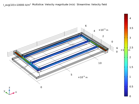
In the Settings window for Streamline, click Replace Expression in the upper-right corner of the Expression section. From the menu, choose Component 1 (comp1) > Brinkman Equations > Velocity and pressure > u,v,w - Velocity field.
|
|
3
|
|
4
|
Locate the Coloring and Style section. Find the Point style subsection. From the Type list, choose Arrow.
|
|
5
|
|
6
|
|
7
|
|
1
|
|
2
|
|
1
|
|
2
|
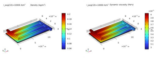
In the Settings window for Surface, click Replace Expression in the upper-right corner of the Expression section. From the menu, choose Component 1 (comp1) > Brinkman Equations > Material properties > br.rho - Density - kg/m³.
|
|
3
|
|
1
|
|
2
|
|
1
|
|
2
|
In the Settings window for Surface, click Replace Expression in the upper-right corner of the Expression section. From the menu, choose Component 1 (comp1) > Brinkman Equations > Material properties > br.mu - Dynamic viscosity - Pa·s.
|
|
3
|
|
1
|
In the Model Builder window, expand the Concentration, H2, Surface (tcs) node, then click Surface 1.
|
|
2
|
|
3
|
|
1
|
In the Model Builder window, expand the Concentration, H2O, Surface (tcs) node, then click Surface 1.
|
|
2
|
|
3
|
|
1
|
|
2
|
|
3
|
|
1
|
|
2
|
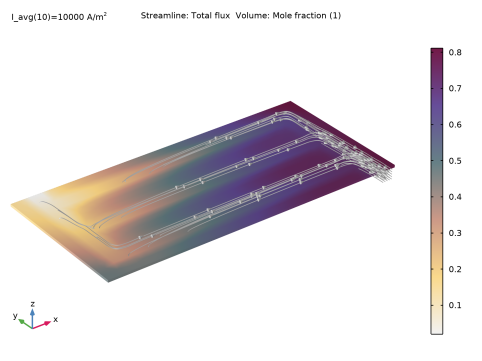
In the Settings window for Streamline, click Replace Expression in the upper-right corner of the Expression section. From the menu, choose Component 1 (comp1) > Transport of Concentrated Species in Porous Media > Species wH2 > Fluxes > tcs.tflux_wH2x,...,tcs.tflux_wH2z - Total flux.
|
|
3
|
|
4
|
|
5
|
Locate the Coloring and Style section. Find the Point style subsection. From the Type list, choose Arrow.
|
|
6
|
|
7
|
|
1
|
|
2
|
|
3
|
|
1
|
|
2
|
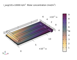
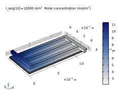
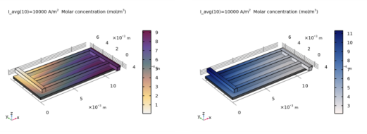
In the Settings window for Volume, click Replace Expression in the upper-right corner of the Expression section. From the menu, choose Component 1 (comp1) > Transport of Concentrated Species in Porous Media > Species wH2 > tcs.x_wH2 - Mole fraction - 1.
|
|
3
|
|
1
|
|
2
|
|
3
|
|
4
|
|
5
|
|
1
|
|
2
|
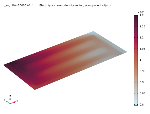
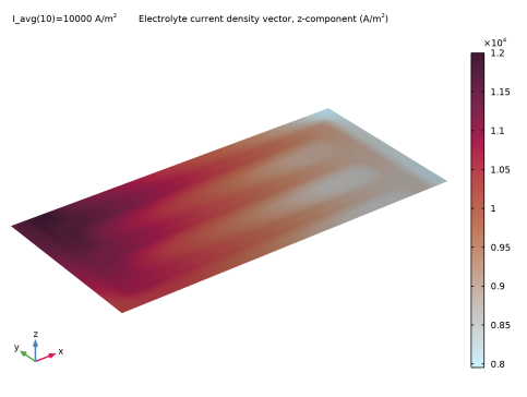
In the Settings window for 3D Plot Group, type Cross-Sectional Electrolyte Current Density in the Label text field.
|
|
3
|
|
1
|
|
2
|
In the Settings window for Slice, click Replace Expression in the upper-right corner of the Expression section. From the menu, choose Component 1 (comp1) > Secondary Current Distribution > Electrolyte current density vector - A/m² > cd.Ilz - Electrolyte current density vector, z-component.
|
|
3
|
|
4
|
|
5
|
|
6
|
|
7
|
|
1
|
|
2
|
|
3
|
|
4
|
|
5
|
|
6
|
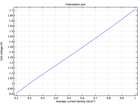
Select the y-axis label checkbox.
|
|
7
|
|
8
|
|
1
|
|
2
|
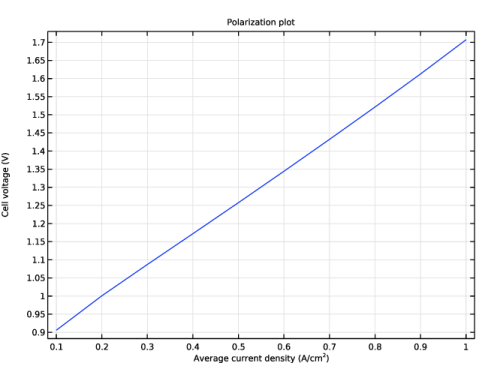
In the Settings window for Global, click Add Expression in the upper-right corner of the y-Axis Data section. From the menu, choose Component 1 (comp1) > Secondary Current Distribution > cd.phis0_ec1 - Electric potential on boundary - V.
|
|
3
|
|
4
|
|
5
|
|
6
|
|
7
|
|
1
|
In the Model Builder window, expand the Concentration, H2, Streamline (tcs) node, then click Streamline 1.
|
|
2
|
|
3
|
|
4
|
Locate the Coloring and Style section. Find the Line style subsection. From the Type list, choose Tube.
|
|
5
|
|
6
|
|
1
|
|
2
|
|
3
|
|
4
|
|
1
|
In the Model Builder window, expand the Concentration, H2O, Streamline (tcs) node, then click Streamline 1.
|
|
2
|
|
3
|
|
4
|
Locate the Coloring and Style section. Find the Line style subsection. From the Type list, choose Tube.
|
|
5
|
|
6
|
|
1
|
|
2
|
|
3
|
|
4
|
|
1
|
In the Model Builder window, under Results, Ctrl-click to select Electrolyte Potential (cd), Electrolyte Current Density (cd), and Electrode Current Density (cd).
|
|
2
|
Right-click and choose Delete.
|
|
1
|
|
2
|
Click
|
|
1
|
|
2
|
|
3
|
|
4
|
Browse to the model’s Application Libraries folder and double-click the file soec_thermodynamics_geom_parameters.txt.
|
|
1
|
|
2
|
|
3
|
|
4
|
|
5
|
|
6
|
Locate the Selections of Resulting Entities section. Select the Resulting objects selection checkbox.
|
|
1
|
|
2
|
|
3
|
|
1
|
|
2
|
|
3
|
|
1
|
|
2
|
|
3
|
|
1
|
|
2
|
|
3
|
|
4
|
|
5
|
|
6
|
|
1
|
Right-click Component 1 (comp1) > Geometry 1 > Work Plane 1 (wp1) > Plane Geometry > Rectangle 1 (r1) and choose Duplicate.
|
|
2
|
|
3
|
|
4
|
|
1
|
|
2
|
|
3
|
|
4
|
|
5
|
|
6
|
|
1
|
|
2
|
Select the object r3 only.
|
|
3
|
|
4
|
|
5
|
|
6
|
|
1
|
|
2
|
|
3
|
Locate the Distances section. In the table, enter the following settings:
|
|
4
|
Locate the Selections of Resulting Entities section. Select the Resulting objects selection checkbox.
|
|
1
|
|
2
|
|
3
|
|
4
|
On the object fin, select Boundary 19 only.
|
|
1
|
|
2
|
|
3
|
|
4
|
On the object fin, select Boundary 42 only.
|
|
1
|
|
2
|
In the Settings window for Explicit Selection, type Cathode Current Collector in the Label text field.
|
|
3
|
|
4
|
On the object fin, select Boundaries 10, 26, 33, and 40 only.
|
|
1
|
|
2
|
In the Settings window for Explicit Selection, type Anode Current Collector in the Label text field.
|
|
3
|
|
4
|
On the object fin, select Boundary 3 only.
|
|
1
|
|
2
|
|
3
|
Click
|
|
4
|
|
5
|
Click OK.
|
|
6
|
In the Settings window for Adjacent Selection, type Channel Domain Boundaries in the Label text field.
|
|
1
|
|
2
|
In the Settings window for Difference Selection, type Boundary Layer Boundaries in the Label text field.
|
|
3
|
|
4
|
|
5
|
|
6
|
Click OK.
|
|
7
|
|
8
|
|
9
|
|
10
|
Click OK.
|