PDF

Water and Carbon Dioxide Co-Electrolysis in a Solid Oxide Electrolyzer Cell
Introduction
In this tutorial, a solid oxide electrolyzer cell model for co-electrolysis of H2O and CO2 is presented. The model includes the full coupling between the mass balances and gas flow in the H2 and O2 gas diffusion electrodes, the momentum balances in the H2 and O2 gas-flow channels, the energy balance across the cell, the balance of the ionic current carried by the oxide ion, and an electronic-current balance. A reversible water–gas shift reaction is included in the H2 gas-diffusion electrode and the H2 gas-flow channel.
The model computes the spatial distributions of the various species across the gas-diffusion electrodes and gas-flow channels. The spatial distribution of the total current density along the electrode length is also evaluated using a general projection operator.
Model Definition
On the anode, oxygen ions are oxidized to form oxygen gas,
(1)
whereas on the cathode, water vapor is reduced to form hydrogen gas and oxygen ions:
(2)
A CO2 electrolysis reaction also occurs on the cathode, where CO2 gas is reduced to form CO gas and oxygen ions:
(3)
Figure 1 shows the model geometry. Seven computational domains are used in the model: the two interconnects, H2 and O2 gas-flow channels, H2 and O2 gas-diffusion electrodes, and the membrane.
Figure 1: Model geometry. From top: Interconnect, H2 gas channel, H2 gas-diffusion electrode, solid oxide electrolyte layer, O2 gas-diffusion electrode, O2 gas-flow channel, and interconnect. The inlet and outlet positions are indicated in the figure.
The gas mixture at the cathode consists of H2, H2O, CO2, and CO, whereas that at the anode consists of O2 and N2. The composition of the gas mixture will change as a result of the electrochemical reactions and the water–gas shift reaction. The mass transport of the gaseous species is modeled in the gas-flow channels and the gas-diffusion electrodes coupled to the resulting (laminar) flow of the gas mixture.
The current distribution is defined assuming a temperature-dependent electrolyte conductivity of the solid electrolyte. The Water Electrolyzer interface is used to define the electrode reactions and the electrolyte charge transport in the porous gas-diffusion electrodes and the electrolyte layer, as well as the mass transport of the gas mixture. The momentum flow is defined using Darcy’s Law in the gas-flow channels and the gas-diffusion electrodes.
On the cathode side, the electrode kinetics depends on the local concentrations of H2O and H2 for the H2O electrolysis reaction and on the local concentrations of CO2 and CO for the CO2 electrolysis reaction according to the law of mass action (and the Nernst equation). On the anode side, the electrode kinetics depends on the local concentrations of O2 for the O2 evolution reaction according to the law of mass action (and the Nernst equation).
The properties of the gas mixtures at both anode and cathode, as well as the equilibrium potentials of the electrode reactions are automatically defined by the default built-in options of the Water Electrolyzer interface.
Results and Discussion
Figure 2 shows the H2 concentration distribution in the H2 gas-flow channel and the H2 gas-diffusion electrode for an applied potential of 1.5 V. The H2 concentration is found to increase along the electrode length due to the H2O electrolysis reaction occurring at the H2 gas diffusion electrode.
Figure 2: H2 concentration distribution in the H2 gas-flow channel and H2 gas-diffusion electrode for an applied potential of 1.5 V.
Figure 3 shows the CO concentration distribution in the H2 gas-flow channel and H2 gas diffusion electrode for applied potential of 1.5 V. CO concentration is found to increase along the electrode length due to the CO2 electrolysis reaction occurring at the H2 gas-diffusion electrode. The difference in the CO concentration between the H2 gas-diffusion electrode and the H2 gas-flow channel is considerably higher for CO in the downstream when compared to H2. This can be attributed to slower diffusion of CO than H2.
Figure 3: CO concentration distribution in the H2 gas-flow channel and the H2 gas-diffusion electrode for an applied potential of 1.5 V.
Figure 4 shows the change in temperature across a solid oxide electrolyzer cell for an applied potential of 1.5 V. Although both the H2O and CO2 electrolysis reactions are endothermic, the cell temperature is increased by about 25 K from the inlet to the outlet for an applied potential of 1.5 V. As this applied potential is higher than the cell thermoneutral potential, the heat generated from overpotential losses is more than the heat required for electrolysis reactions.
Figure 4: Change in temperature across a solid oxide electrolyzer cell for an applied potential of 1.5 V.
Figure 5 shows the distribution of the water–gas shift reaction rate in the H2 gas-flow channel and the H2 gas-diffusion electrode for an applied potential of 1.5 V. The water–gas shift reaction rate is found to be higher closer to the H2 gas-diffusion electrode-membrane interface for an applied potential of 1.5 V, which is attributed to the high CO concentration in the region.
Figure 5: Water–gas shift reaction rate in the H2 gas-flow channel and the H2 gas-diffusion electrode for an applied potential of 1.5 V.
Figure 6 shows that the total cathodic (negative) current density, which is integrated along the y direction for each grid point along the x direction using a general projection operator, decreases for H2O electrolysis and increases for CO2 electrolysis along the electrode length.
Figure 6: The total cathodic current density for H2O and CO2 electrolysis along the electrode length for an applied potential of 1.5 V.
Finally, Figure 7 shows the average current density as a function of the applied potential (polarization curve).
Figure 7: Polarization curve.
Application Library path: Fuel_Cell_and_Electrolyzer_Module/Electrolyzers/soec_co2
Modeling Instructions
From the File menu, choose New.
New
In the New window, click  Model Wizard.
Model Wizard
1
In the Model Wizard window, click  2D.
2
In the Select Physics tree, select Electrochemistry > Water Electrolyzers > Solid Oxide (we).
3
Click Add.
4
In the Select Physics tree, select Heat Transfer > Heat Transfer in Solids and Fluids (ht).
5
Click Add.
6
Click  Study.
7
In the Select Study tree, select Preset Studies for Selected Physics Interfaces > Water Electrolyzer > Stationary with Initialization.
8
Global Definitions
Parameters 1
First load the model parameters.
1
In the Model Builder window, under Global Definitions click Parameters 1.
2
In the Settings window for Parameters, locate the Parameters section.
3
Click  Load from File.
4
Geometry 1
Draw the model geometry using a rectangle and six layers.
1
In the Sketch toolbar, click Rectangle and choose Rectangle.
Rectangle 1 (r1)
1
In the Model Builder window, expand the Geometry 1 node.
2
Right-click Component 1 (comp1) > Geometry 1 and choose Rectangle.
3
In the Settings window for Rectangle, locate the Size and Shape section.
4
In the Width text field, type L.
5
In the Height text field, type W.
6
Click to expand the Layers section. In the table, enter the following settings:
7
Click  Build All Objects.
Definitions
Variables 1
Next, add variables.
1
In the Definitions toolbar, click  Local Variables.
2
In the Settings window for Variables, locate the Variables section.
3
Click  Load from File.
4
General Projection 1 (genproj1)
Next, add a General Projection coupling.
1
In the Definitions toolbar, click  Nonlocal Couplings and choose General Projection.
2
Average 1 (aveop1)
Add an average operator which will be used later while plotting the polarization plot.
1
In the Definitions toolbar, click  Nonlocal Couplings and choose Average.
2
In the Settings window for Average, type aveop_an in the Operator name text field.
3
Locate the Source Selection section. From the Geometric entity level list, choose Boundary.
4
Water Electrolyzer (we)
Start setting up the electrochemistry part of the model.
1
In the Model Builder window, under Component 1 (comp1) click Water Electrolyzer (we).
2
3
In the Settings window for Water Electrolyzer, locate the H2 Gas Mixture section.
4
Select the CO2 checkbox.
5
Select the CO checkbox.
6
Find the Transport mechanisms subsection. Select the Use Darcy’s Law for momentum transport checkbox.
7
Locate the O2 Gas Mixture section. Select the N2 checkbox.
8
Select the Include gas phase diffusion checkbox.
9
Select the Use Darcy’s Law for momentum transport checkbox.
Membrane 1
1
In the Physics toolbar, click  Domains and choose Membrane.
2
H2 Gas Diffusion Electrode 1
1
In the Physics toolbar, click  Domains and choose H2 Gas Diffusion Electrode.
2
3
In the Settings window for H2 Gas Diffusion Electrode, locate the Effective Electrolyte Charge Transport section.
4
In the εl text field, type epsl.
5
Locate the Gas Transport section. From the Effective diffusivity correction list, choose Tortuosity.
6
In the εg text field, type epsg.
7
In the τg text field, type taug.
8
In the κg text field, type kappag_GDE.
H2 Gas Diffusion Electrode Reaction: Water Electrolysis
1
In the Model Builder window, under Component 1 (comp1) > Water Electrolyzer (we) > H2 Gas Diffusion Electrode 1 click H2 Gas Diffusion Electrode Reaction 1.
2
In the Settings window for H2 Gas Diffusion Electrode Reaction, type H2 Gas Diffusion Electrode Reaction: Water Electrolysis in the Label text field.
3
Locate the Electrode Kinetics section. In the i0,ref(T) text field, type i0_ref_HER.
4
In the αa text field, type 0.5.
5
Locate the Active Specific Surface Area section. In the av text field, type S.
H2 Gas Diffusion Electrode 1
In the Model Builder window, click H2 Gas Diffusion Electrode 1.
H2 Gas Diffusion Electrode Reaction: CO2 Electrolysis
1
In the Physics toolbar, click  Attributes and choose H2 Gas Diffusion Electrode Reaction.
2
In the Settings window for H2 Gas Diffusion Electrode Reaction, type H2 Gas Diffusion Electrode Reaction: CO2 Electrolysis in the Label text field.
3
Locate the Stoichiometric Coefficients section. In the νCO2 text field, type -1.
4
In the νCO text field, type 1.
5
Locate the Electrode Kinetics section. In the i0,ref(T) text field, type i0_ref_COER.
6
Locate the Active Specific Surface Area section. In the av text field, type S.
O2 Gas Diffusion Electrode 1
1
In the Physics toolbar, click  Domains and choose O2 Gas Diffusion Electrode.
2
3
In the Settings window for O2 Gas Diffusion Electrode, locate the Effective Electrolyte Charge Transport section.
4
In the εl text field, type epsl.
5
Locate the Gas Transport section. From the Effective diffusivity correction list, choose Tortuosity.
6
In the εg text field, type epsg.
7
In the τg text field, type taug.
8
In the κg text field, type kappag_GDE.
O2 Gas Diffusion Electrode Reaction 1
1
In the Model Builder window, click O2 Gas Diffusion Electrode Reaction 1.
2
In the Settings window for O2 Gas Diffusion Electrode Reaction, locate the Electrode Kinetics section.
3
In the i0,ref(T) text field, type i0_ref_OER.
4
Locate the Active Specific Surface Area section. In the av text field, type S.
H2 Gas Flow Channel 1
Next, add the H2 Gas Flow Channel.
1
In the Physics toolbar, click  Domains and choose H2 Gas Flow Channel.
2
3
In the Settings window for H2 Gas Flow Channel, locate the Gas Transport section.
4
From the list, choose Straight channels.
5
In the H text field, type dg.
6
In the W text field, type dg.
O2 Gas Flow Channel 1
Next, add the O2 Gas Flow Channel.
1
In the Physics toolbar, click  Domains and choose O2 Gas Flow Channel.
2
3
In the Settings window for O2 Gas Flow Channel, locate the Gas Transport section.
4
From the list, choose Straight channels.
5
In the H text field, type dg.
6
In the W text field, type dg.
Electronic Conducting Phase 1
Next, specify the initial values for the oxygen domain to enhance convergence and set the boundary conditions.
1
In the Model Builder window, click Electronic Conducting Phase 1.
Initial Values, O2 Domains 1
1
In the Physics toolbar, click  Attributes and choose Initial Values, O2 Domains.
2
3
In the Settings window for Initial Values, O2 Domains, locate the Initial Values section.
4
In the ϕs text field, type E_app.
Electronic Conducting Phase 1
In the Model Builder window, click Electronic Conducting Phase 1.
Electric Ground 1
1
In the Physics toolbar, click  Attributes and choose Electric Ground.
2
Electronic Conducting Phase 1
In the Model Builder window, click Electronic Conducting Phase 1.
Electric Potential 1
1
In the Physics toolbar, click  Attributes and choose Electric Potential.
2
3
In the Settings window for Electric Potential, locate the Electric Potential section.
4
In the ϕs,bnd text field, type E_app.
H2 Gas Phase 1
Next, specify initial values, add the water gas shift reaction, and set the hydrogen inlet and outlet boundary conditions.
Initial Values 1
1
In the Model Builder window, click Initial Values 1.
2
In the Settings window for Initial Values, locate the Initial Composition section.
3
In the x0,H2O text field, type x0_H2O.
4
In the x0,CO2 text field, type x0_CO2.
5
In the x0,CO text field, type x0_CO.
H2 Gas Phase 1
In the Model Builder window, click H2 Gas Phase 1.
Water Gas Shift Reaction 1
1
In the Physics toolbar, click  Attributes and choose Water Gas Shift Reaction.
2
In the Settings window for Water Gas Shift Reaction, locate the Water Gas Shift Reaction Rate section.
3
In the kWGSR text field, type k_wgsr.
4
In the pref text field, type 1[Pa].
H2 Gas Phase 1
In the Model Builder window, click H2 Gas Phase 1.
H2 Inlet 1
1
In the Physics toolbar, click  Attributes and choose H2 Inlet.
2
3
In the Settings window for H2 Inlet, locate the Inlet Flow Type section.
4
Clear the Stoichiometric feed checkbox.
5
Locate the Mass Flow Rates section. In the J0,H2O text field, type Mflux_in*w0_H2O.
6
In the J0,CO2 text field, type Mflux_in*w0_CO2.
7
In the J0,CO text field, type Mflux_in*w0_CO.
8
Locate the Flow Boundary Condition section. From the list, choose Total mass flow rate.
9
In the J0 text field, type Mflux_in.
H2 Gas Phase 1
In the Model Builder window, click H2 Gas Phase 1.
H2 Outlet 1
1
In the Physics toolbar, click  Attributes and choose H2 Outlet.
2
O2 Gas Phase 1
Next, set the initial values and the oxygen inlet and outlet boundary conditions.
Initial Values 1
1
In the Model Builder window, click Initial Values 1.
2
In the Settings window for Initial Values, locate the Initial Composition section.
3
In the x0,N2 text field, type x0_N2.
O2 Gas Phase 1
In the Model Builder window, click O2 Gas Phase 1.
O2 Inlet 1
1
In the Physics toolbar, click  Attributes and choose O2 Inlet.
2
3
In the Settings window for O2 Inlet, locate the Inlet Flow Type section.
4
From the Inlet flow type list, choose Mass flow rates.
5
Locate the Mass Flow Rates section. In the J0,N2 text field, type Mflux_in*w0_N2.
6
Locate the Flow Boundary Condition section. From the list, choose Total mass flow rate.
7
In the J0 text field, type Mflux_in.
O2 Gas Phase 1
In the Model Builder window, click O2 Gas Phase 1.
O2 Outlet 1
1
In the Physics toolbar, click  Attributes and choose O2 Outlet.
2
Heat Transfer in Solids and Fluids (ht)
Next, set the heat transfer physics.
1
In the Model Builder window, under Component 1 (comp1) click Heat Transfer in Solids and Fluids (ht).
2
In the Settings window for Heat Transfer in Solids and Fluids, locate the Physical Model section.
3
In the Tref text field, type T_in.
Solid: Interconnects
1
In the Model Builder window, under Component 1 (comp1) > Heat Transfer in Solids and Fluids (ht) click Solid 1.
2
In the Settings window for Solid, type Solid: Interconnects in the Label text field.
Fluid: Flow Channels
1
In the Model Builder window, under Component 1 (comp1) > Heat Transfer in Solids and Fluids (ht) click Fluid 1.
2
In the Settings window for Fluid, type Fluid: Flow Channels in the Label text field.
3
4
Locate the Model Input section. From the pA list, choose User defined. In the associated text field, type we.pA.
5
Locate the Heat Convection section. Specify the u vector as
6
Locate the Heat Conduction, Fluid section. From the k list, choose Thermal conductivity, gas phase (we).
7
Locate the Thermodynamics, Fluid section. From the Fluid type list, choose Gas/Liquid.
8
From the ρ list, choose Density of gas phase (we).
9
From the Cp list, choose Heat capacity at constant pressure, gas phase (we).
Initial Values 1
1
In the Model Builder window, click Initial Values 1.
2
In the Settings window for Initial Values, locate the Initial Values section.
3
In the T text field, type T_in.
Porous Medium: Cathode GDE
Next, add thermal conductivities for the gas diffusion electrode domains.
1
In the Physics toolbar, click  Domains and choose Porous Medium.
2
In the Settings window for Porous Medium, type Porous Medium: Cathode GDE in the Label text field.
3
Fluid 1
1
In the Model Builder window, click Fluid 1.
2
In the Settings window for Fluid, locate the Model Input section.
3
From the pA list, choose User defined. In the associated text field, type we.pA.
4
Locate the Heat Convection section. Specify the u vector as
5
Locate the Heat Conduction, Fluid section. From the kf list, choose Thermal conductivity, gas phase (we).
6
Locate the Thermodynamics, Fluid section. From the ρf list, choose Density of gas phase (we).
7
From the Cp,f list, choose Heat capacity at constant pressure, gas phase (we).
Porous Matrix 1
1
In the Model Builder window, click Porous Matrix 1.
2
In the Settings window for Porous Matrix, locate the Matrix Properties section.
3
From the εp list, choose User defined. In the associated text field, type epsg.
4
Locate the Heat Conduction, Porous Matrix section. From the kb list, choose User defined. In the associated text field, type kc.
5
Locate the Thermodynamics, Porous Matrix section. From the ρb list, choose User defined. From the Cp,b list, choose User defined.
Porous Medium: Anode GDE
1
In the Physics toolbar, click  Domains and choose Porous Medium.
2
In the Settings window for Porous Medium, type Porous Medium: Anode GDE in the Label text field.
3
Fluid 1
1
In the Model Builder window, click Fluid 1.
2
In the Settings window for Fluid, locate the Model Input section.
3
From the pA list, choose User defined. In the associated text field, type we.pA.
4
Locate the Heat Convection section. Specify the u vector as
5
Locate the Heat Conduction, Fluid section. From the kf list, choose Thermal conductivity, gas phase (we).
6
Locate the Thermodynamics, Fluid section. From the ρf list, choose Density of gas phase (we).
7
From the Cp,f list, choose Heat capacity at constant pressure, gas phase (we).
Porous Matrix 1
1
In the Model Builder window, click Porous Matrix 1.
2
In the Settings window for Porous Matrix, locate the Matrix Properties section.
3
From the εp list, choose User defined. In the associated text field, type epsg.
4
Locate the Heat Conduction, Porous Matrix section. From the kb list, choose User defined. In the associated text field, type ka.
5
Locate the Thermodynamics, Porous Matrix section. From the ρb list, choose User defined. From the Cp,b list, choose User defined.
Solid: Membrane
Next, add thermal conductivity for the membrane domains.
1
In the Physics toolbar, click  Domains and choose Solid.
2
In the Settings window for Solid, type Solid: Membrane in the Label text field.
3
4
Locate the Heat Conduction, Solid section. From the k list, choose User defined. In the associated text field, type km.
5
Locate the Thermodynamics, Solid section. From the ρ list, choose User defined. From the Cp list, choose User defined.
Inflow 1
Next, add the inflow, outflow, and periodic condition boundary conditions.
1
In the Physics toolbar, click  Boundaries and choose Inflow.
2
3
In the Settings window for Inflow, locate the Upstream Properties section.
4
In the Tustr text field, type T_in.
Outflow 1
1
In the Physics toolbar, click  Boundaries and choose Outflow.
2
Periodic Condition 1
1
In the Physics toolbar, click  Boundaries and choose Periodic Condition.
2
Multiphysics
Next, add an electrochemical heating multiphysics coupling.
Electrochemical Heating 1 (ech1)
In the Physics toolbar, click  Multiphysics Couplings and choose Domain > Electrochemical Heating.
Materials
Now, add materials from the Material Library.
Add Material
1
In the Materials toolbar, click  Add Material to open the Add Material window.
2
Go to the Add Material window.
3
In the tree, select Fuel Cell and Electrolyzer > Solid Oxides > Yttria-Stabilized Zirconia, 8YSZ, (ZrO2)0.92-(Y2O3)0.08.
4
Click the Add to Component button in the window toolbar.
Materials
Yttria-Stabilized Zirconia, 8YSZ, (ZrO2)0.92-(Y2O3)0.08 (mat1)
1
In the Settings window for Material, locate the Geometric Entity Selection section.
2
Click  Clear Selection.
3
Add Material
1
Go to the Add Material window.
2
In the tree, select Built-in > Steel AISI 4340.
3
Click the Add to Component button in the window toolbar.
4
In the Materials toolbar, click  Add Material to close the Add Material window.
Materials
Steel AISI 4340 (mat2)
Select Domains 1 and 7 only.
Mesh 1
Next, set up a user-controlled mesh.
Distribution 1
1
In the Model Builder window, under Component 1 (comp1) right-click Mesh 1 and choose Distribution.
2
3
In the Settings window for Distribution, locate the Distribution section.
4
In the Number of elements text field, type 100.
Distribution 2
1
In the Model Builder window, right-click Mesh 1 and choose Distribution.
2
3
In the Settings window for Distribution, locate the Distribution section.
4
In the Number of elements text field, type 2.
Distribution 3
1
Right-click Mesh 1 and choose Distribution.
2
3
In the Settings window for Distribution, locate the Distribution section.
4
In the Number of elements text field, type 10.
Distribution 4
1
Right-click Mesh 1 and choose Distribution.
2
3
In the Settings window for Distribution, locate the Distribution section.
4
In the Number of elements text field, type 2.
Distribution 5
1
Right-click Mesh 1 and choose Distribution.
2
3
In the Settings window for Distribution, locate the Distribution section.
4
From the Distribution type list, choose Predefined.
5
In the Number of elements text field, type 20.
6
In the Element ratio text field, type 10.
7
From the Growth rate list, choose Exponential.
Distribution 6
1
Right-click Mesh 1 and choose Distribution.
2
3
In the Settings window for Distribution, locate the Distribution section.
4
From the Distribution type list, choose Predefined.
5
In the Number of elements text field, type 10.
6
In the Element ratio text field, type 5.
7
From the Growth rate list, choose Exponential.
8
Select the Reverse direction checkbox.
Mapped 1
1
In the Mesh toolbar, click  Mapped.
2
In the Settings window for Mapped, click  Build All.
3
Click the  Zoom Extents button in the Graphics toolbar.
The mesh should look like this:
Study 1
Finally, set the study settings using an auxiliary sweep for the applied potential to complete the model setup.
Step 1: Current Distribution Initialization
1
In the Model Builder window, under Study 1 click Step 1: Current Distribution Initialization.
2
In the Settings window for Current Distribution Initialization, locate the Study Settings section.
3
From the Current distribution type list, choose Secondary.
Step 2: Stationary
1
In the Model Builder window, click Step 2: Stationary.
2
In the Settings window for Stationary, click to expand the Study Extensions section.
3
Select the Auxiliary sweep checkbox.
4
5
6
In the Study toolbar, click  Compute.
Results
Some plots are added by default. Follow the instructions below to reproduce the figures in the Results and Discussion section.
Surface 1
1
In the Model Builder window, expand the Mole Fraction, H2 (we) node, then click Surface 1.
2
In the Settings window for Surface, locate the Coloring and Style section.
3
From the Color table list, choose ConopiformisZero.
Streamline 1
1
In the Model Builder window, click Streamline 1.
2
In the Settings window for Streamline, locate the Streamline Positioning section.
3
In the Density level text field, type 7.
4
Locate the Coloring and Style section. Find the Point style subsection. From the Arrow length list, choose Proportional.
5
From the Color list, choose Cyan.
6
In the Mole Fraction, H2 (we) toolbar, click  Plot.
The plot should look like Figure 2.
Surface 1
1
In the Model Builder window, expand the Mole Fraction, CO (we) node, then click Surface 1.
2
In the Settings window for Surface, locate the Coloring and Style section.
3
From the Color table list, choose ConopiformisZero.
Streamline 1
1
In the Model Builder window, click Streamline 1.
2
In the Settings window for Streamline, locate the Streamline Positioning section.
3
In the Density level text field, type 7.5.
4
Locate the Coloring and Style section. Find the Point style subsection. From the Arrow length list, choose Proportional.
5
From the Color list, choose Cyan.
6
In the Mole Fraction, CO (we) toolbar, click  Plot.
The plot should look like Figure 3.
Surface 1
1
In the Model Builder window, expand the Temperature (ht) node, then click Surface 1.
2
In the Settings window for Surface, locate the Expression section.
3
In the Expression text field, type T-T_in.
Temperature (ht)
1
In the Model Builder window, click Temperature (ht).
2
In the Settings window for 2D Plot Group, click to expand the Title section.
3
From the Title type list, choose Manual.
4
In the Title text area, type Surface: Change in Temperature (K).
5
In the Temperature (ht) toolbar, click  Plot.
The plot should look like Figure 4.
Water Gas Shift Reaction Rate
Next, plot the water gas shift reaction rate over the hydrogen gas diffusion electrode and flow channel domains.
1
In the Results toolbar, click  2D Plot Group.
2
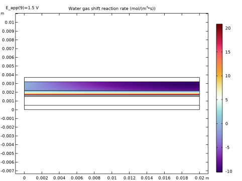
In the Settings window for 2D Plot Group, type Water Gas Shift Reaction Rate in the Label text field.
Surface 1
1
In the Water Gas Shift Reaction Rate toolbar, click  Surface.
2
In the Settings window for Surface, locate the Expression section.
3
In the Expression text field, type we.r_wgsr.
4
Locate the Coloring and Style section. From the Color table list, choose Ctenophora.
5
In the Water Gas Shift Reaction Rate toolbar, click  Plot.
The plot should look like Figure 5.
Current Density Distribution
Add a plot for the total integrated current density across the electrode length.
1
In the Results toolbar, click  1D Plot Group.
2
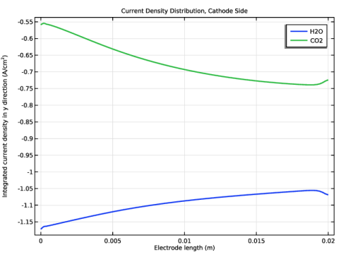
In the Settings window for 1D Plot Group, type Current Density Distribution in the Label text field.
3
Locate the Data section. From the Parameter selection (E_app) list, choose Last.
4
Click to expand the Title section. From the Title type list, choose Manual.
5
In the Title text area, type Current Density Distribution, Cathode Side.
6
Locate the Plot Settings section.
7
Select the x-axis label checkbox. In the associated text field, type Electrode length (m).
8
Select the y-axis label checkbox. In the associated text field, type Integrated current density in y direction (A/cm<sup>2</sup>).
Line Graph 1
1
In the Current Density Distribution toolbar, click  Line Graph.
2
3
In the Settings window for Line Graph, locate the y-Axis Data section.
4
In the Expression text field, type genproj1(we.iv_h2gder1).
5
In the Unit field, type A/cm^2.
6
Click to expand the Coloring and Style section. From the Width list, choose 2.
7
Click to expand the Legends section. Select the Show legends checkbox.
8
From the Legends list, choose Manual.
9
Current Density Distribution
In the Model Builder window, click Current Density Distribution.
Line Graph 2
1
In the Current Density Distribution toolbar, click  Line Graph.
2
3
In the Settings window for Line Graph, locate the y-Axis Data section.
4
In the Expression text field, type genproj1(we.iv_h2gder2).
5
In the Unit field, type A/cm^2.
6
Locate the Coloring and Style section. From the Width list, choose 2.
7
Locate the Legends section. Select the Show legends checkbox.
8
From the Legends list, choose Manual.
9
Current Density Distribution
1
In the Model Builder window, click Current Density Distribution.
2
In the Current Density Distribution toolbar, click  Plot.
The plot should look like Figure 6.
Polarization Plot
Finally, add the Polarization Plot.
1
In the Home toolbar, click  Add Plot Group and choose 1D Plot Group.
2
In the Settings window for 1D Plot Group, type Polarization Plot in the Label text field.
3
Click to expand the Title section. From the Title type list, choose Manual.
4
In the Title text area, type Polarization plot.
5
Locate the Plot Settings section. Select the x-axis label checkbox.
6
Select the y-axis label checkbox.
7
In the x-axis label text field, type Applied potential (V).
8
In the y-axis label text field, type Average current density (A/cm<sup>2</sup>).
Point Graph 1
1
Right-click Polarization Plot and choose Point Graph.
2
3
In the Settings window for Point Graph, locate the y-Axis Data section.
4
In the Expression text field, type aveop_an(we.nIs).
5
In the Unit field, type A/cm^2.
6
Click to expand the Coloring and Style section. From the Width list, choose 2.
7
Click to expand the Legends section. Clear the Show legends checkbox.
8
In the Polarization Plot toolbar, click  Plot.
The plot should look like Figure 7.
Follow the commands below to improve the appearance of the other plots.
Surface 1
1
In the Model Builder window, expand the Electrode Potential with Respect to Ground (we) node, then click Surface 1.
2
In the Settings window for Surface, locate the Coloring and Style section.
3
From the Color table list, choose MetasepiaBlue.
Arrow Surface 1
In the Model Builder window, right-click Arrow Surface 1 and choose Disable.
Surface 1
1
In the Model Builder window, expand the Electrolyte Potential (we) node, then click Surface 1.
2
In the Settings window for Surface, locate the Coloring and Style section.
3
From the Color table list, choose MetasepiaBlue.
Arrow Surface 1
1
In the Model Builder window, click Arrow Surface 1.
2
In the Settings window for Arrow Surface, locate the Coloring and Style section.
3
From the Color list, choose Yellow.
Surface 1
1
In the Model Builder window, expand the Mole Fraction, O2 (we) node, then click Surface 1.
2
In the Settings window for Surface, locate the Coloring and Style section.
3
From the Color table list, choose ConopiformisZero.
Streamline 1
1
In the Model Builder window, click Streamline 1.
2
In the Settings window for Streamline, locate the Streamline Positioning section.
3
In the Density level text field, type 8.
4
Locate the Coloring and Style section. Find the Point style subsection. From the Arrow length list, choose Proportional.
5
From the Color list, choose Cyan.
Surface 1
1
In the Model Builder window, expand the Mole Fraction, H2O (we) node, then click Surface 1.
2
In the Settings window for Surface, locate the Coloring and Style section.
3
From the Color table list, choose ConopiformisZero.
Streamline 1
1
In the Model Builder window, click Streamline 1.
2
In the Settings window for Streamline, locate the Streamline Positioning section.
3
In the Density level text field, type 9.
4
Locate the Coloring and Style section. Find the Point style subsection. From the Arrow length list, choose Proportional.
5
From the Color list, choose Cyan.
Surface 1
1
In the Model Builder window, expand the Mole Fraction, N2 (we) node, then click Surface 1.
2
In the Settings window for Surface, locate the Coloring and Style section.
3
From the Color table list, choose ConopiformisZero.
Streamline 1
1
In the Model Builder window, click Streamline 1.
2
In the Settings window for Streamline, locate the Streamline Positioning section.
3
In the Density level text field, type 8.
4
Locate the Coloring and Style section. Find the Point style subsection. From the Arrow length list, choose Proportional.
5
From the Color list, choose Cyan.
Surface 1
1
In the Model Builder window, expand the Mole Fraction, CO2 (we) node, then click Surface 1.
2
In the Settings window for Surface, locate the Coloring and Style section.
3
From the Color table list, choose ConopiformisZero.
Streamline 1
1
In the Model Builder window, click Streamline 1.
2
In the Settings window for Streamline, locate the Streamline Positioning section.
3
In the Density level text field, type 8.
4
Locate the Coloring and Style section. Find the Point style subsection. From the Arrow length list, choose Proportional.
5
From the Color list, choose Cyan.
Surface 1
1
In the Model Builder window, expand the Pressure (we) node, then click Surface 1.
2
In the Settings window for Surface, locate the Coloring and Style section.
3
From the Color table list, choose HelfrichiZero.
4
From the Color table type list, choose Discrete.
Streamline 1
1
In the Model Builder window, click Streamline 1.
2
In the Settings window for Streamline, locate the Streamline Positioning section.
3
In the Density level text field, type 9.
4
Locate the Coloring and Style section. Find the Point style subsection. From the Arrow length list, choose Proportional.
5
From the Color list, choose Gray.