|
|
|
|
1
|
|
2
|
In the Select Physics tree, select Electrochemistry > Water Electrolyzers > Proton Exchange Membrane (we).
|
|
3
|
Click Add.
|
|
4
|
Click
|
|
5
|
In the Select Study tree, select Preset Studies for Selected Physics Interfaces > Stationary with Initialization.
|
|
6
|
Click
|
|
1
|
|
2
|
|
3
|
Click
|
|
4
|
Browse to the model’s Application Libraries folder and double-click the file pemwe_1d_parameters.txt.
|
|
1
|
|
2
|
|
3
|
|
1
|
|
2
|
|
3
|
|
5
|
|
1
|
|
2
|
Go to the Add Material window.
|
|
3
|
In the tree, select Fuel Cell and Electrolyzer > Polymer Electrolytes > Nafion®, EW 1100, Liquid Equilibrated, Protonated.
|
|
4
|
Right-click and choose Add to Component 1 (comp1).
|
|
5
|
|
6
|
|
1
|
|
2
|
|
3
|
|
4
|
|
1
|
|
3
|
|
4
|
|
1
|
|
3
|
|
4
|
|
1
|
|
1
|
|
3
|
|
4
|
|
1
|
|
2
|
In the Settings window for Thin H2 Gas Diffusion Electrode Reaction, locate the Electrode Kinetics section.
|
|
3
|
|
4
|
|
1
|
|
3
|
|
4
|
|
1
|
|
2
|
In the Settings window for Thin O2 Gas Diffusion Electrode Reaction, locate the Electrode Kinetics section.
|
|
3
|
|
4
|
|
1
|
|
1
|
|
3
|
|
4
|
|
1
|
In the Model Builder window, under Component 1 (comp1) > Water Electrolyzer (we) click H2 Gas Phase 1.
|
|
2
|
|
3
|
|
4
|
|
5
|
|
1
|
|
2
|
|
3
|
|
4
|
|
5
|
|
1
|
|
2
|
|
3
|
|
4
|
|
5
|
|
6
|
|
1
|
|
2
|
|
3
|
Select the Auxiliary sweep checkbox.
|
|
4
|
Click
|
|
6
|
Click
|
|
7
|
|
8
|
|
9
|
|
10
|
Click Replace.
|
|
11
|
|
1
|
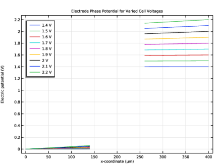
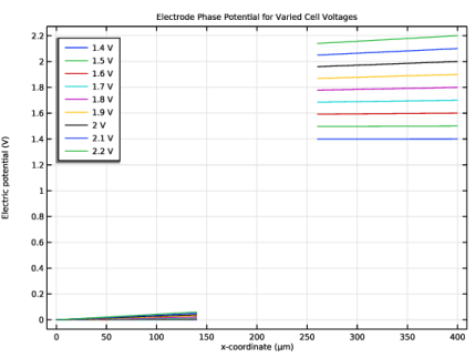
In the Settings window for 1D Plot Group, type Electrode Phase Potential for Varied Cell Voltages in the Label text field.
|
|
2
|
|
3
|
|
1
|
In the Model Builder window, expand the Electrode Phase Potential for Varied Cell Voltages node, then click Line Graph 1.
|
|
2
|
|
3
|
Select the Show legends checkbox.
|
|
4
|
|
1
|
|
2
|
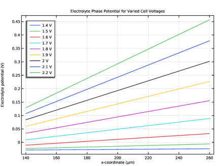
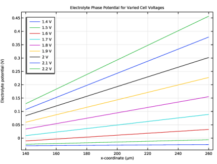
In the Settings window for 1D Plot Group, type Electrolyte Phase Potential for Varied Cell Voltages in the Label text field.
|
|
3
|
|
4
|
|
1
|
In the Model Builder window, expand the Electrolyte Phase Potential for Varied Cell Voltages node, then click Line Graph 1.
|
|
2
|
|
3
|
Select the Show legends checkbox.
|
|
4
|
|
1
|
|
2
|
|
1
|
|
3
|
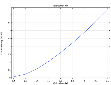
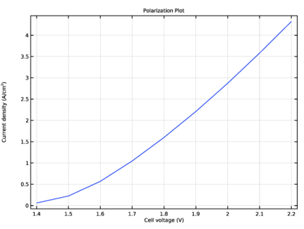
In the Settings window for Point Graph, click Replace Expression in the upper-right corner of the y-Axis Data section. From the menu, choose Component 1 (comp1) > Water Electrolyzer > we.nIs - Normal electrode current density - A/m².
|
|
4
|
|
5
|
|
1
|
|
2
|
|
3
|
|
4
|
Locate the Plot Settings section.
|
|
5
|
|
6
|
Select the y-axis label checkbox. In the associated text field, type Current density (A/cm<sup>2</sup>).
|
|
7
|
|
1
|
|
2
|
|
1
|
|
3
|
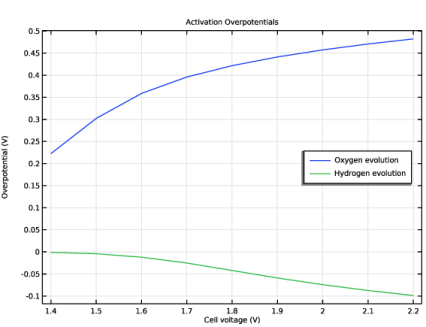
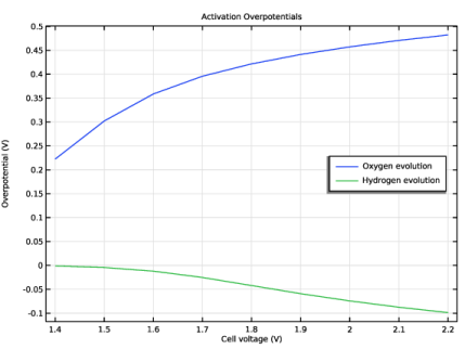
In the Settings window for Point Graph, click Replace Expression in the upper-right corner of the y-Axis Data section. From the menu, choose Component 1 (comp1) > Water Electrolyzer > Electrode kinetics > we.eta_to2gder1 - Overpotential - V.
|
|
4
|
|
5
|
|
1
|
|
3
|
In the Settings window for Point Graph, click Replace Expression in the upper-right corner of the y-Axis Data section. From the menu, choose Component 1 (comp1) > Water Electrolyzer > Electrode kinetics > we.eta_th2gder1 - Overpotential - V.
|
|
4
|
|
5
|
|
1
|
|
2
|
|
3
|
|
4
|
Locate the Plot Settings section.
|
|
5
|
|
6
|
|
7
|