COMSOL 6.4 - Parameter Estimation of a Polymer Electrolyte Membrane Fuel Cell Model

Parameter Estimation of a Polymer Electrolyte Membrane Fuel Cell Model

This tutorial demonstrates how to use stationary polarization data to perform parameter estimation of a polymer electrolyte membrane fuel cell (PEMFC) model. The model, defining a 5-layer membrane electrode assembly (MEA) is two-dimensional and includes electronic and ionic charge balances, Butler–Volmer kinetics, as well as gas diffusive and convective transport in the oxygen/air gas diffusion layer and electrode (catalytic layer).

Two sets of polarization data, for either a humidified oxygen or air mixture, are used for estimation of four model parameters.

The experimental data and most of the parameters used for defining the model are based on Ref. 1.

Model Definition

Figure 1 shows the model geometry. The geometry consists of five layers: two gas diffusion layers (GDLs), two gas diffusion electrodes (catalytic layers), and one membrane. The left-hand side upper and lower boundaries represent the boundaries facing the ribs of the flow-field plates, acting as current collectors. The right-hand side upper and lower boundaries represent the boundaries facing the gas flow channels, acting as gas inlet/outlets. The upper side of the cell is the oxygen/air side (cathode) side; the lower side is the hydrogen (anode) side.

The two-dimensional geometry can be motivated by assuming that the gases are fed to the cell at high stoichiometry (flow rates) so that partial pressure gradients are negligible along the channels.

Figure 1: Model geometry of the 5-layer MEA. A membrane, sandwiched between two catalytic layer (gas diffusion electrode) domains, is located between the two gas diffusion layers. The points indicate the intersection between the rib and channels outside the model geometry.

The model is defined using the interface, including the following phenomena:

•

Electronic and ionic charge balances using Ohm’s law.

•

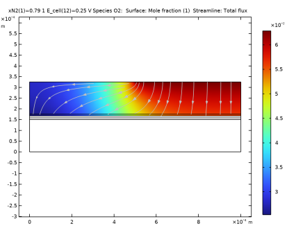
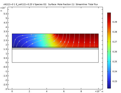
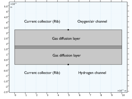
Gas diffusion and convection of the O2/N2/H2O mixture on the oxygen side of the cell in the corresponding GDL and the catalytic layer. (For this cell configuration, hydrogen transport will be fast and it is assumed the partial pressure gradients on the hydrogen side are negligible.)

•

Butler–Volmer kinetics in the catalytic layers. On the oxygen side, the kinetics depends on the local partial pressure of oxygen and water vapor. In addition, a local limiting current density is incorporated on the oxygen side representing additional concentration overpotentials due to diffusion through a thin ionomer film covering the catalyst particles.

•

Hydrogen permeation through the membrane, giving rise to a small parasitic current on the catalytic layer/membrane boundary on the oxygen side.

For an introduction to fuel cell MEA modeling, see also the Transport Phenomena in a Polymer Electrolyte Fuel Cell Membrane Electrode Assembly tutorial.

Parameter estimation

The study step is used to fit the model to the experimental polarization data. The stationary polarization data, recorded for both a humidified oxygen and a humidified air oxidant stream, is shown in Figure 2. When using the humidified oxygen as oxidant, the current densities are generally higher.

Figure 2: Experimental polarization data.

At high cell voltages, the polarization curves feature a nonlinear voltage dependency on the current density. This nonlinearity is usually associated with kinetic losses, for PEMFCs in particular to the sluggish oxygen reduction reaction (ORR). At intermediate cell voltages, where ohmic voltage losses dominate the polarization behavior, the graphs are more linear. For low voltages, in particular for the air case, the curves bend off downward, approaching a limiting current density, which stems from transport limitations.

In order to achieve a good model fit to the data, we choose a set of fitting parameters that will impact all these three regions of the polarization data. The fitting parameters (also called control variables) are summarized in Table 1.

Table 1: Fitting Parameters.
Name	Unit	Description
sigmal_mem	S/m	Membrane electrolyte conductivity
log_i0_ref_ORR	-	Log of oxygen reduction reference exchange current density
alphac_ORR	-	Cathodic transfer coefficient for oxygen reduction
ilim_ORR_ref	A/m2	Limiting current density for oxygen reduction at 1 atm partial pressure

The parameter sigmal_mem defines the electrolyte conductivity of the membrane. This parameter contributes to the linear voltage dependency and will hence affect the slope of the polarization curves in the linear region.

The parameters log_i0_ref_ORR and alphac_ORR are used in the Butler–Volmer kinetics expression on the oxygen side of the cell, and will mainly affect the upper, nonlinear, region of the polarization plots. Note that we choose to fit the log of the exchange current density, rather than the exchange current density variable directly. In this way, negative values are inherently avoided, and it is also easier to get a good fit if the initial guess of the fitting parameter is off by orders of magnitudes.

The final parameter, ilim_ORR_ref, is also used in the kinetics expression on the oxygen side, but will only affect the kinetics expression for large current densities. This parameter will hence affect the lower, transport-limited, part of the polarization curves.

Results and Discussion

Figure 3 shows the results of the fitted model, along with the experimental polarization data.

Figure 3: Polarization plots for oxygen (green) and air (blue). Solid lines: fitted model. Markers: experimental data.

The corresponding fitted parameter values are shown in Table 2.

Table 2: Fitted Parameter values.
Name	Unit	Initial guess	Fitted Value
sigmal_mem	S/m	10	3.8
log_i0_ref_ORR	-	-3	-3.5
alphac_ORR	-	0.74	0.91
ilim_ORR_ref	A/m2	3000	2.2e3

Reference

1. M. Butori, B. Eriksson, N. Nikolic, C. Lagergren , G. Lindbergh, and R. Wreland Lindström, “The effect of oxygen partial pressure and humidification in proton exchange membrane fuel cells at intermediate temperature (80–120ºC),” J. Power Sources, vol. 563, p. 232803, 2023.

Fuel_Cell_and_Electrolyzer_Module/Fuel_Cells/pemfc_parameter_estimation

Modeling Instructions

From the menu, choose .

New

In the window, click

Model Wizard

In the window, click

In the tree, select > > .

Click .

Click

In the tree, select > .

Click

Global Definitions

Parameters 1

Load the model parameters from a text file.

In the window, under click .

In the window for , locate the section.

Click

Browse to the model’s Application Libraries folder and double-click the file pemfc_parameter_estimation_parameters.txt.

Geometry 1

Draw the gas diffusion layers, the catalyst layers and the membrane of the five-layer fuel cell membrane-electrode-assembly (MEA) as individual rectangles in the geometry. By enabling the , the resulting domains become available as named selections later on when defining the physics.

Hydrogen GDL

In the toolbar, click

In the window for , type Hydrogen GDL in the text field.

Locate the section. In the text field, type W_cell.

In the text field, type H_gdl.

Locate the section. Select the checkbox.

Click

Hydrogen Catalyst Layer

In the toolbar, click

In the window for , type Hydrogen Catalyst Layer in the text field.

Locate the section. In the text field, type W_cell.

In the text field, type H_ct.

Locate the section. In the text field, type H_gdl.

Locate the section. Select the checkbox.

Click

Membrane

In the toolbar, click

In the window for , type Membrane in the text field.

Locate the section. In the text field, type W_cell.

In the text field, type H_mem.

Locate the section. In the text field, type H_gdl+H_ct.

Locate the section. Select the checkbox.

Click

Oxygen Catalyst Layer

In the toolbar, click

In the window for , type Oxygen Catalyst Layer in the text field.

Locate the section. In the text field, type W_cell.

In the text field, type H_ct.

Locate the section. In the text field, type H_gdl+H_ct+H_mem.

Locate the section. Select the checkbox.

Click

Oxygen GDL

In the toolbar, click

In the window for , type Oxygen GDL in the text field.

Locate the section. In the text field, type W_cell.

In the text field, type H_gdl.

Locate the section. In the text field, type H_gdl+H_ct+H_mem+H_ct.

Locate the section. Select the checkbox.

Click

Point 1 (pt1)

Add points to divide the upper and lower boundaries at the intersection between the ribs and the channels.

In the toolbar, click

In the window for , locate the section.

In the text field, type W_rib/2.

Click

Point 2 (pt2)

Right-click and choose .

In the window for , locate the section.

In the text field, type H_cell.

Click

In the toolbar, click

Click the

button in the toolbar.

The final geometry should now look as follows:

Definitions

Variables 1

In the window, under right-click and choose .

Load some variable expressions from a text file.

In the window for , locate the section.

Click

Browse to the model’s Application Libraries folder and double-click the file pemfc_parameter_estimation_variables.txt.

One of the variable expressions indicate an unknown operator or function. Add the missing integration operator as follows:

Integration 1 (intop1)

In the toolbar, click

and choose .

This operator will be used to compute an integral along the top current collector.

In the window for , type intop_cc in the text field.

Locate the section. From the list, choose .

Enable to facilitate boundary selection.

In the window, click .

In the window for , locate the section.

Select the checkbox.

Integration 1 (intop_cc)

In the window, click .

Select Boundary 11 only.

Variables 1

If you defined the operator correctly, the indication for the missing operator should now have vanished.

Hydrogen Fuel Cell (fc)

Now proceed to define the fuel cell model.

In the window, under click .

In the window for , locate the section.

Find the subsection. Clear the checkbox.

Locate the section. Select the checkbox.

Click to expand the section. Find the subsection. Select the checkbox.

H2 Gas Diffusion Electrode 1

In the toolbar, click

and choose .

In the window for , locate the section.

From the list, choose .

Locate the section. In the σs text field, type sigmas_ct.

Locate the section. From the list, choose . In the fl text field, type 1.

In this model we will assume the electrolyte conductivity defined on the node always refers to the effective electrolyte conductivity. Hence the correction factor is set to unity.

H2 Gas Diffusion Electrode Reaction 1

In the window, click .

In the window for , locate the section.

In the i0,ref(T) text field, type i0_ref_HOR.

Locate the section. In the av text field, type Av_HOR.

O2 Gas Diffusion Electrode 1

In the toolbar, click

and choose .

In the window for , locate the section.

From the list, choose .

Locate the section. In the σs text field, type sigmas_ct.

Locate the section. From the list, choose . In the fl text field, type 1.

Locate the section. In the εg text field, type epsg_ct.

In the κg text field, type perm_ct.

O2 Gas Diffusion Electrode Reaction 1

In the window, click .

In the window for , locate the section.

In the i0,ref(T) text field, type i0_ref_ORR.

In the αa text field, type alphaa_ORR.

This models adds a limiting current density, representing the oxygen mass transport limitations in a thin ionomer film, covering the catalytic particles.

Select the checkbox.

In the ilim text field, type ilim_ORR.

Locate the section. In the av text field, type Av_ORR.

H2 Gas Diffusion Layer 1

In the toolbar, click

and choose .

In the window for , locate the section.

From the list, choose .

Specify different conductivity values in the x and y directions as follows.

Locate the section. From the list, choose .

Specify the σs matrix as


sigmas_gdl_IP	0
0	sigmas_gdl_TP

O2 Gas Diffusion Layer 1

In the toolbar, click

and choose .

In the window for , locate the section.

From the list, choose .

Locate the section. From the list, choose .

Specify the σs matrix as


sigmas_gdl_IP	0
0	sigmas_gdl_TP

Locate the section. In the εg text field, type epsg_gdl.

In the κg text field, type perm_gdl.

Membrane 1

In the toolbar, click

and choose .

In the window for , locate the section.

From the list, choose .

Locate the section. From the ΨH2 list, choose . In the associated text field, type perm_H2.

Electrolyte Phase 1

Add a second node to define the effective conductivity of the membrane. Thereby the default node will be refer to the catalytic layers only.

In the window, click .

In the window for , locate the section.

From the σl list, choose . In the associated text field, type sigmal_mem.

Electrolyte Phase 2

In the toolbar, click

and choose .

Select Domains 2 and 4 only.

In the window for , locate the section.

From the σl list, choose . In the associated text field, type sigmal_ct.

Electronic Conducting Phase 1

In the window, click .

Electric Ground 1

In the toolbar, click

and choose .

Select Boundary 2 only.

Electronic Conducting Phase 1

In the window, click .

Electric Potential 1

In the toolbar, click

and choose .

Select Boundary 11 only.

In the window for , locate the section.

In the ϕs,bnd text field, type E_cell.

Electronic Conducting Phase 1

Specify the initial electrode phase potential on the oxygen side. This improves convergence.

In the window, click .

Initial Values, O2 Domains 1

In the toolbar, click

and choose .

In the window for , locate the section.

From the list, choose .

Locate the section. In the ϕs text field, type E_init.

H2 Gas Phase 1

In the window, under > click .

In the window for , locate the section.

From the list, choose .

In the RHhum text field, type RH.

In the Thum text field, type T.

Initial Values 1

In the window, under > > click .

In the window for , locate the section.

From the list, choose .

In the RHhum text field, type RH.

In the Thum text field, type T.

O2 Gas Phase 1

In the window, click .

O2 Inlet 1

In the toolbar, click

and choose .

Select Boundary 13 only.

In the window for , locate the section.

From the list, choose .

Locate the section. From the list, choose .

In the x0,N2,dry text field, type xN2.

In the RHhum text field, type RH.

In the Thum text field, type T.

Global Definitions

Default Model Inputs

The temperature defined on the will be used by all physics nodes.

In the window, under click .

In the window for , locate the section.

In the tree, select > .

Find the subsection. In the text field, type T.

Mesh 1

Define a user-defined mesh as follows:

In the window, under click .

In the window for , locate the section.

From the list, choose .

In the toolbar, click

Mapped 1

In the toolbar, click

In the window for , locate the section.

From the list, choose .

Select Domains 2–4 only.

Distribution 1

Right-click and choose .

Select Boundaries 3 and 15 only.

In the window for , locate the section.

From the list, choose .

In the text field, type 5.

Select the checkbox.

Distribution 2

In the window, right-click and choose .

Select Boundaries 5 and 16 only.

In the window for , locate the section.

In the text field, type 2.

Distribution 3

Right-click and choose .

Select Boundaries 7 and 17 only.

Free Triangular 1

In the toolbar, click

Size 1

Right-click and choose .

In the window for , locate the section.

From the list, choose .

Select Points 7 and 8 only.

Locate the section. From the list, choose .

Click

The finalized mesh should now look as follows:

The problem is now ready for solving. Enable an to perform polarization sweeps for two different dry inlet nitrogen molar fractions.

Study 1

Parametric Sweep

In the toolbar, click

In the window for , locate the section.

Click

In the table, enter the following settings:


Parameter name	Parameter value list	Parameter unit
xN2 (Dry nitrogen molar fraction)	0.79 0	1

A dry nitrogen molar fraction of 0.79 corresponds to air, 0 to pure oxygen.

In the table, click to select the cell at row number 1 and column number 3.

Click to expand the section. From the list, choose .

Step 1: Stationary

For each nitrogen leve, enable an to perform a sweep of the cell potential.

In the window, click .

In the window for , click to expand the section.

Select the checkbox.

Click

In the table, enter the following settings:


Parameter name	Parameter value list	Parameter unit
E_cell (Cell voltage)	range(E_init,-0.05,0.25)	V

Note that is set to by default. This improves convergence since this will result in that, for each nitrogen level, the potential will swept from a higher to a lower value, using the result of the previous computation as initial values for each step.

In the toolbar, click

Results

Mole Fraction, O2 (fc)

You may now explore the default plots for various nitrogen and cell voltage levels.

In the window, under click .

In the window for , locate the section.

From the list, choose .

In the toolbar, click

From the list, choose .

In the toolbar, click

Polarization Plots

Add a polarization plots for air and oxygen as follows:

In the toolbar, click

In the window for , locate the section.

From the list, choose .

In the text field, type Polarization Plots.

Global 1

Right-click and choose .

In the window for , locate the section.

In the table, enter the following settings:


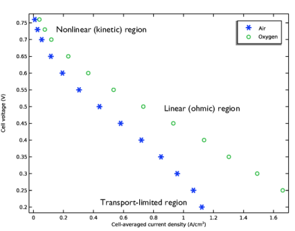
Expression	Unit	Description
E_cell	V	Cell voltage

Click in the upper-right corner of the section. From the menu, choose > > > .

Locate the section. In the field, type A/cm^2.

Click to expand the section. From the list, choose .

In the table, enter the following settings:


Legends
Air
Oxygen

Polarization Plots

In the window, click .

In the window for , click to expand the section.

From the list, choose .

In the toolbar, click

Table 1 - Air Polarization Data

The next step is to compare the computed polarization plots to the corresponding experimental data. Import the polarization data as a table and plot it as follows:

In the toolbar, click

In the window for , type Table 1 - Air Polarization Data in the text field.

Locate the section. Click

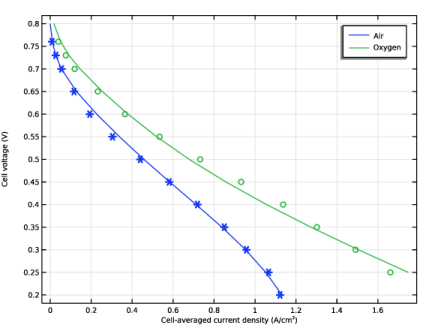
Browse to the model’s Application Libraries folder and double-click the file pemfc_parameter_estimation_air_data.csv.

Table 2 - O2 Polarization Data

In the toolbar, click

In the window for , type Table 2 - O2 Polarization Data in the text field.

Locate the section. Click

Browse to the model’s Application Libraries folder and double-click the file pemfc_parameter_estimation_o2_data.csv.

Polarization Plots

Enable the x- and y-axis label checkboxes at this point. This will avoid the upcoming table graphs to impact the axis labels.

In the window, under click .

In the window for , locate the section.

Select the checkbox.

Table Graph 1

Right-click and choose .

In the window for , locate the section.

Find the subsection. From the list, choose .

From the list, choose .

Find the subsection. From the list, choose .

Table Graph 2

Right-click and choose .

In the window for , locate the section.

From the list, choose .

Locate the section. From the list, choose .

In the toolbar, click

Component 1 (comp1)

The model captures the overall trends in the polarization data, but the model predictivity is poor. In this second part of the tutorial, we will use to improve the model. operates by minimizing objective functions using an optimization solver.

Global Least-Squares Objective - Air

The nodes will create objective functions based on the data tables, where in this tutorial the columns are defined as either a or a column. Each objective function is defined as a sum for all rows of the squared differences between experimental data values and the corresponding model variable values, as defined by the columns and the associated settings. For each row in the data, model parameters may be varied to the values defined in the columns.

Multiple nodes may be used, and additional model parameters may be varied for each node, as set by the section.

How the objective functions are to be minimized will be defined later when we set up the study.

In the toolbar, click

and choose .

In the window for , type Global Least-Squares Objective - Air in the text field.

Locate the section. From the list, choose .

Locate the section. In the table, enter the following settings:


Columns	Type	Settings
Current Density (mA/cm^2)	Value	Model expression=I_cell_avg, Column name=col1

In the text field, type I_cell_avg.

In the text field, type A/cm^2.

In the table, enter the following settings:


Columns	Type	Settings
Cell Voltage (V)	Parameter	Name=E_cell

From the list, choose .

In the text field, type V.

Locate the section. Click

In the table, enter the following settings:


Name	Expression
xN2 (Dry nitrogen molar fraction)	0.79

Global Least-Squares Objective - Oxygen

Right-click and choose .

In the window for , type Global Least-Squares Objective - Oxygen in the text field.

Locate the section. From the list, choose .

Locate the section. In the table, enter the following settings:


Name	Expression
xN2 (Dry nitrogen molar fraction)	0

Add Study

Add a second study to perform parameter estimation.

In the toolbar, click

to open the window.

Go to the window.

Find the subsection. In the tree, select > .

Click the button in the window toolbar.

In the toolbar, click

to close the window.

Study 2

Parameter Estimation

In the toolbar, click

and choose .

Note that the least-square objectives you defined earlier are now selected by automatically in the section. This means that the sum of the two least-squares functions will subject to minimization.

In the section you define what parameters to modify (fit) in order to minimize the objective function, together with (optional) bounds. For this model we will estimate the values of four parameters.

In the window for , locate the section.

Click

In the table, enter the following settings:


Parameter	Initial value	Scale	Lower bound	Upper bound	Unit
sigmal_mem (Membrane electrolyte conductivity)	10[S/m]	1	1	20	S/m

Click

In the table, enter the following settings:


Parameter	Initial value	Scale	Lower bound	Upper bound	Unit
log10_i0_ref_ORR (Log of ORR reference exchange current density (fitting parameter))	-3	1	-6	0

Click

In the table, enter the following settings:


Parameter	Initial value	Scale	Lower bound	Upper bound	Unit
alphac_ORR (Cathodic transfer coefficient, oxygen reduction)	log(10)R_constT/(100[mV]*F_const)	0.1	0.5	1	1

Click

In the table, enter the following settings:


Parameter	Initial value	Scale	Lower bound	Upper bound	Unit
ilim_ORR_ref (Limiting current density for oxygen reduction at 1 atm partial pressure)	3000[A/m^2]	1000	1000	5000	A/m^2

Locate the section. From the list, choose .

Step 1: Stationary

By enabling an , we guide the sweep to start at a high voltage, and then gradually lower the voltage. As in , by running continuation for the cell voltage parameter, this improves convergence.

In the window, click .

In the window for , locate the section.

Select the checkbox.

From the list, choose .

In the text field, type E_init.

In the toolbar, click