PDF

Carbon Corrosion in a Polymer Electrolyte Membrane Fuel Cell
Introduction
Carbon corrosion is one of the important degradation mechanisms in polymer electrolyte membrane (PEM) fuel cells. It predominantly occurs during start up or shut down of the cell. During carbon corrosion, the noble-metal-catalyst carbon support is compromised, affecting the cell performance.
In this model, a shut-down air purging scenario is modeled by introducing air in a flow channel on the hydrogen (H2) side, at the same as one of the channels on the H2 side remains filled with H2. This situation may for instance occur if a gas flow channel on the H2 side is clogged by a water droplet during air purging.
Model Definition
Figure 1 shows the model geometry. Three computational domains are used in the model: H2 and O2 gas-diffusion layers (GDL), and the membrane. Thin H2 and O2 gas-diffusion electrodes, H2 inlets, electrode current and electric ground boundary conditions are also shown in Figure 1.
Figure 1: Model geometry. From top: O2 gas-diffusion layer, Membrane and H2 gas-diffusion layer. Thin O2 gas-diffusion electrode, Thin H2 gas-diffusion electrode, H2 inlets, Electrode current and Electric ground boundary conditions are indicated in the figure.
The gas mixture at the anode consists of H2, H2O, N2, and O2, whereas that at the cathode consists of O2, H2O, N2, and CO2. The mass transport of the gaseous species and momentum transport using Darcy’s Law is modeled for the H2 gas mixture whereas a constant gas mixture (humidified air) is assumed for the O2 gas mixture.
The Hydrogen Fuel Cell interface is used to define the electrode reactions, the electrolyte charge transport in the electrolyte layer, the electrode charge transport in the porous gas-diffusion layers, as well as the mass transport of the H2 GDL.
The top boundary of the O2 GDL in Figure 1 is facing O2 gas channel and the bottom boundary of the H2 GDL is facing H2 gas channel. Note that gas channels are not explicitly defined as domains in the geometry; instead they are represented by boundary conditions. H2 is fed from the right bottom boundary of the H2 GDL whereas air is fed from the left bottom boundary of the H2 GDL using a ramp function to introduce air gradually with time. A zero electrode current is set at the top middle boundary of the O2 GDL, and the bottom middle boundary of the H2 GDL is grounded. Although the net current of the cell is 0, internal current circulation exists in the cell due to local potential variation within the cell. The Thin H2 and O2 gas-diffusion electrodes define electrode kinetics for the electrochemical reactions considered in the model.
On the H2 side (anode during normal operation), the hydrogen oxidation (HOR) and oxygen reduction (ORR) reactions are considered at the Thin H2 gas diffusion electrode:
(1)
(2)
whereas on the O2 side (cathode during normal operation), the oxygen reduction (ORR) and carbon oxidation (COR) reactions are considered at the Thin O2 gas diffusion electrode:
(3)
(4)
On the H2 side, the electrode kinetics depends on the local concentrations of H2 for the HOR and on the local concentrations of H2O and O2 for the ORR according to the Butler-Volmer kinetics (and the Nernst equation). On the O2 side, the electrode kinetics depends on the local concentrations of H2O and O2 for the ORR and on H2O and CO2 for the COR according to the Butler-Volmer kinetics (and the Nernst equation).
The properties of the gas mixtures at both sides, as well as the equilibrium potentials of the electrode reactions (except for the COR) are automatically defined by the default built-in options of the Hydrogen Fuel Cell interface.
Hydrogen Cross-over Transport Through the Membrane
Hydrogen diffusing from the anode side through the membrane is assumed to be oxidized as soon as it reaches the cathode catalytic layer according to
(5)
Assuming the hydrogen concentration to be zero at the membrane-cathode catalytic boundary and in equilibrium with gaseous hydrogen on the anode side, the flux of hydrogen though the membrane is defined as
(6)
where ΨH2 (SI unit: m2/s) is the hydrogen permeation coefficient in the ionomer (incorporating the hydrogen gas-ionomer phase transfer partition constant) and Lmem is the membrane thickness.
The hydrogen oxidation current is added to the charge balance as a boundary electrolyte current density contribution
(7)
The model uses the three study steps: Current Distribution Initialization, Stationary and Time dependent. Secondary current distribution type is used in the Current Distribution Initialization study step. The stationary study step solves for H2 side without air and the Time dependent study solves for H2 side with gradually introduced air.
Results and Discussion
Figure 2 shows the change in the cell voltage versus time. It can be seen that the cell voltage is almost uniform at the beginning, before suddenly dropping to its new steady-state of around 0.88 V at around 1 s. This sudden drop in the cell voltage is attributed to the carbon oxidation reaction occurring in the oxygen-side of the cell, as discussed later.
Figure 2: Cell voltage versus time.
Figure 3 shows the H2 mole-fraction distribution in the H2 gas-diffusion layer at t = 1.2 s.
Figure 3: H2 mole-fraction distribution in the H2 gas-diffusion layer at t = 1.2 s.
Figure 4 shows the O2 mole-fraction distribution in the H2 and O2 gas-diffusion layers at t = 1.2 s. The presence of oxygen in the anode domain is due to humidified air fed into the anode domain from one end, mimicking shut-down operation of the fuel cell.
Figure 4: O2 mole-fraction distribution in the H2 and O2 gas-diffusion layers at t = 1.2 s.
Figure 5 shows the change in the hydrogen-side electrode potential along the length of the fuel cell for different times. The hydrogen-side electrode potential increases with time before attaining a maximum steady-state potential of around 0.7 V at around 1 s.
Figure 5: Change in the hydrogen-side electrode potential along the length of the fuel cell.
Figure 6 shows the change in the oxygen-side electrode potential along the length of the fuel cell for different times. The oxygen-side electrode potential increases with time before attaining a maximum steady state potential of around 1.55 V at around 1 s.
Figure 6: Change in the oxygen-side electrode potential along the length of the fuel cell.
Figure 7 shows the change in the carbon corrosion rate, which is evaluated from the local current density for the carbon oxidation reaction, along the length of the fuel cell for different times. The carbon corrosion rate increases with time and is found to be at its peak at around 1 s. The carbon corrosion is also found to occur in the region where humidified air is fed in the hydrogen-side of the fuel cell.
Figure 7: Change in the carbon corrosion rate along the length of the fuel cell.
Figure 8 shows the change in the hydrogen-side local current density along the length of the fuel cell at t = 1.2 s. It can be seen that both the hydrogen oxidation and oxygen reduction reactions occur, particularly at the interface between hydrogen and air, at the Thin H2 gas-diffusion electrodes node.
Figure 8: Change in the hydrogen-side current density along the length of the fuel cell.
Finally, Figure 9 shows the change in the oxygen-side local current density for the oxygen reduction and carbon oxidation reactions and the total current density along the length of the fuel cell at t = 1.2 s. It can be seen that the oxygen reduction reaction occurs at the Thin O2 gas-diffusion electrodes node in the region where hydrogen is fed whereas the oxygen evolution reaction occurs in the region where humidified air is fed in the hydrogen-side of the fuel cell.
Figure 9: Change in the oxygen-side current density along the length of the fuel cell.
Application Library path: Fuel_Cell_and_Electrolyzer_Module/Fuel_Cells/pemfc_carbon_corrosion
Modeling Instructions
From the File menu, choose New.
New
In the New window, click  Model Wizard.
Model Wizard
1
In the Model Wizard window, click  2D.
2
In the Select Physics tree, select Electrochemistry > Hydrogen Fuel Cells > Proton Exchange Membrane (fc).
3
Click Add.
4
Click  Study.
5
In the Select Study tree, select Preset Studies for Selected Physics Interfaces > Stationary with Initialization.
6
Global Definitions
Parameters 1
First load the model parameters.
1
In the Model Builder window, under Global Definitions click Parameters 1.
2
In the Settings window for Parameters, locate the Parameters section.
3
Click  Load from File.
4
Geometry 1
The model geometry consists of three domains: the hydrogen-side gas diffusion layer (GDL), the membrane, and the oxygen-side GDL.
1
In the Model Builder window, under Component 1 (comp1) click Geometry 1.
2
In the Settings window for Geometry, locate the Units section.
3
From the Length unit list, choose mm.
4
In the Sketch toolbar, click Rectangle and choose Rectangle.
H2 Gas-Diffusion Layer
1
In the Model Builder window, expand the Geometry 1 node.
2
Right-click Component 1 (comp1) > Geometry 1 and choose Rectangle.
3
In the Settings window for Rectangle, type H2 Gas-Diffusion Layer in the Label text field.
4
Locate the Size and Shape section. In the Width text field, type W_rib+W_ch.
5
In the Height text field, type H_gdl.
6
Locate the Selections of Resulting Entities section. Select the Resulting objects selection checkbox.
Membrane
1
In the Geometry toolbar, click  Rectangle.
2
In the Settings window for Rectangle, type Membrane in the Label text field.
3
Locate the Size and Shape section. In the Width text field, type W_rib+W_ch.
4
In the Height text field, type H_mem.
5
Locate the Position section. In the y text field, type H_gdl.
6
Locate the Selections of Resulting Entities section. Select the Resulting objects selection checkbox.
O2 Gas-Diffusion Layer
1
In the Geometry toolbar, click  Rectangle.
2
In the Settings window for Rectangle, type O2 Gas-Diffusion Layer in the Label text field.
3
Locate the Size and Shape section. In the Width text field, type W_rib+W_ch.
4
In the Height text field, type H_gdl.
5
Locate the Position section. In the y text field, type H_gdl+H_mem.
6
Locate the Selections of Resulting Entities section. Select the Resulting objects selection checkbox.
7
In the Sketch toolbar, click  Point.
Point 1 (pt1)
1
In the Geometry toolbar, click  Point.
2
In the Settings window for Point, locate the Point section.
3
In the x text field, type W_ch/2.
Point 2 (pt2)
1
In the Geometry toolbar, click  Point.
2
In the Settings window for Point, locate the Point section.
3
In the x text field, type W_ch/2+W_rib.
Copy 1 (copy1)
1
In the Geometry toolbar, click  Transforms and choose Copy.
2
Select the objects pt1 and pt2 only.
3
In the Settings window for Copy, locate the Displacement section.
4
In the y text field, type 2*H_gdl+H_mem.
5
Click  Build Selected.
6
Click the  Zoom Extents button in the Graphics toolbar.
Definitions
Variables 1
Next, add variables.
1
In the Definitions toolbar, click  Local Variables.
2
In the Settings window for Variables, locate the Variables section.
3
Click  Load from File.
4
Materials
Add the polymer electrolyte material from the material library. The material added will be used by the Electrolyte Phase node to define the conductivity of the electrolyte and by the Membrane node to define the permeation coefficient of the membrane.
Add Material
1
In the Materials toolbar, click  Add Material to open the Add Material window.
2
Go to the Add Material window.
3
In the tree, select Fuel Cell and Electrolyzer > Polymer Electrolytes > Nafion®, EW 1100, Vapor Equilibrated, Protonated.
4
Right-click and choose Add to Component 1 (comp1).
5
In the Materials toolbar, click  Add Material to close the Add Material window.
Hydrogen Fuel Cell (fc)
Set up the current distribution and transport model. Include mass transport using Maxwell-Stefan diffusion and momentum transport using Darcy’s Law in the anode gas mixture. A constant gas mixture (humidified air) is assumed on the cathode side. Additionally, include crossover of hydrogen in the membrane. Note that the default gas species are hydrogen, water, nitrogen and oxygen on the anode side, and oxygen, water, nitrogen and carbon dioxide on the cathode side. Start with adding the relevant domain nodes.
1
In the Settings window for Hydrogen Fuel Cell, locate the H2 Gas Mixture section.
2
Select the N2 checkbox.
3
Select the O2 checkbox.
4
Find the Transport mechanisms subsection. Select the Use Darcy’s Law for momentum transport checkbox.
5
Locate the O2 Gas Mixture section. Select the CO2 checkbox.
6
Clear the Include gas phase diffusion checkbox.
7
Click to expand the Electrolyte and Membrane Transport section. Find the Crossover species subsection. Select the H2 checkbox.
Membrane 1
1
In the Physics toolbar, click  Domains and choose Membrane.
2
In the Settings window for Membrane, locate the Domain Selection section.
3
From the Selection list, choose Membrane.
4
Locate the Electrolyte Water Activity for Material Model Input section. In the aw text field, type 0.95.
H2 Gas Diffusion Layer 1
1
In the Physics toolbar, click  Domains and choose H2 Gas Diffusion Layer.
Set up the properties of the anode gas-diffusion layer in the H2 Gas-Diffusion Layer node.
2
In the Settings window for H2 Gas Diffusion Layer, locate the Domain Selection section.
3
From the Selection list, choose H2 Gas-Diffusion Layer.
4
Locate the Electrode Charge Transport section. In the σs text field, type sigmas_GDL.
5
Locate the Gas Transport section. In the εg text field, type epsg_GDL.
6
In the κg text field, type kappag_GDL.
O2 Gas Diffusion Layer 1
1
In the Physics toolbar, click  Domains and choose O2 Gas Diffusion Layer.
Set up the properties of the cathode gas-diffusion layer in the O2 Gas-Diffusion Layer node.
2
In the Settings window for O2 Gas Diffusion Layer, locate the Domain Selection section.
3
From the Selection list, choose O2 Gas-Diffusion Layer.
4
Locate the Electrode Charge Transport section. In the σs text field, type sigmas_GDL.
Thin H2 Gas Diffusion Electrode 1
Set up the properties of the Thin H2 Gas Diffusion Electrode node. The details of electrode kinetics are set in the child nodes. Note that the reference equilibrium potential is calculated automatically when the default Built in option is used.
1
In the Physics toolbar, click  Boundaries and choose Thin H2 Gas Diffusion Electrode.
2
3
In the Settings window for Thin H2 Gas Diffusion Electrode, locate the Electrode Thickness section.
4
In the dgde text field, type H_gde.
Thin H2 Gas-Diffusion Electrode Reaction - HOR
1
In the Model Builder window, under Component 1 (comp1) > Hydrogen Fuel Cell (fc) > Thin H2 Gas Diffusion Electrode 1 click Thin H2 Gas Diffusion Electrode Reaction 1.
2
In the Settings window for Thin H2 Gas Diffusion Electrode Reaction, type Thin H2 Gas-Diffusion Electrode Reaction - HOR in the Label text field.
3
Locate the Electrode Kinetics section. In the i0,ref(T) text field, type i0_ref_HOR.
4
Locate the Active Specific Surface Area section. In the av text field, type Av_Pt_H2_side.
Thin H2 Gas Diffusion Electrode 1
In the Model Builder window, click Thin H2 Gas Diffusion Electrode 1.
Thin H2 Gas-Diffusion Electrode Reaction - ORR
1
In the Physics toolbar, click  Attributes and choose Thin H2 Gas Diffusion Electrode Reaction.
2
In the Settings window for Thin H2 Gas Diffusion Electrode Reaction, type Thin H2 Gas-Diffusion Electrode Reaction - ORR in the Label text field.
3
Locate the Stoichiometric Coefficients section. In the n text field, type 4.
4
In the νO2 text field, type -1.
5
In the νH2O text field, type 2.
6
Locate the Electrode Kinetics section. From the Exchange current density type list, choose Lumped multistep.
7
In the i0,ref(T) text field, type i0_ref_ORR.
8
From the Pressure dependence list, choose Cathodic reaction orders.
9
In the ξc,O2 text field, type 1.
10
Locate the Active Specific Surface Area section. In the av text field, type Av_Pt_H2_side.
Thin O2 Gas Diffusion Electrode 1
Set up the properties of the Thin O2 Gas-Diffusion Electrode node. The details of electrode kinetics are set in the child nodes.
1
In the Physics toolbar, click  Boundaries and choose Thin O2 Gas Diffusion Electrode.
2
3
In the Settings window for Thin O2 Gas Diffusion Electrode, locate the Electrode Thickness section.
4
In the dgde text field, type H_gde.
Thin O2 Gas-Diffusion Electrode Reaction - ORR
1
In the Model Builder window, under Component 1 (comp1) > Hydrogen Fuel Cell (fc) > Thin O2 Gas Diffusion Electrode 1 click Thin O2 Gas Diffusion Electrode Reaction 1.
2
In the Settings window for Thin O2 Gas Diffusion Electrode Reaction, type Thin O2 Gas-Diffusion Electrode Reaction - ORR in the Label text field.
3
Locate the Electrode Kinetics section. From the Exchange current density type list, choose Lumped multistep.
4
In the i0,ref(T) text field, type i0_ref_ORR.
5
From the Pressure dependence list, choose Cathodic reaction orders.
6
In the ξc,O2 text field, type 1.
7
In the αa text field, type 0.5.
8
Locate the Active Specific Surface Area section. In the av text field, type Av_Pt_O2_side.
Thin O2 Gas Diffusion Electrode 1
In the Model Builder window, click Thin O2 Gas Diffusion Electrode 1.
Thin O2 Gas-Diffusion Electrode Reaction - COR
1
In the Physics toolbar, click  Attributes and choose Thin O2 Gas Diffusion Electrode Reaction.
2
In the Settings window for Thin O2 Gas Diffusion Electrode Reaction, type Thin O2 Gas-Diffusion Electrode Reaction - COR in the Label text field.
3
Locate the Stoichiometric Coefficients section. In the n text field, type 4.
4
In the νH2O text field, type 2.
5
In the νCO2 text field, type -1.
6
Locate the Equilibrium Potential section. From the Eeq,ref(T) list, choose User defined. In the associated text field, type Eeq_COR.
7
Locate the Electrode Kinetics section. In the i0,ref(T) text field, type i0_ref_COR.
8
Locate the Active Specific Surface Area section. In the av text field, type Av_C.
Electronic Conducting Phase 1
Next, specify the initial values for the oxygen domain to enhance convergence and set the boundary conditions.
1
In the Model Builder window, under Component 1 (comp1) > Hydrogen Fuel Cell (fc) click Electronic Conducting Phase 1.
Initial Values, O2 Domains 1
1
In the Physics toolbar, click  Attributes and choose Initial Values, O2 Domains.
2
Electronic Conducting Phase 1
In the Model Builder window, click Electronic Conducting Phase 1.
Electric Ground 1
1
In the Physics toolbar, click  Attributes and choose Electric Ground.
2
Electronic Conducting Phase 1
In the Model Builder window, click Electronic Conducting Phase 1.
Electrode Current 1
1
In the Physics toolbar, click  Attributes and choose Electrode Current.
2
3
In the Settings window for Electrode Current, locate the Electrode Current section.
4
In the Is,total text field, type 0[A].
Next, specify initial values, and set the hydrogen inlet boundary conditions.
Initial Values 1
1
In the Model Builder window, under Component 1 (comp1) > Hydrogen Fuel Cell (fc) > H2 Gas Phase 1 click Initial Values 1.
2
In the Settings window for Initial Values, locate the Initial Composition section.
3
From the Mixture specification list, choose Humidified mixture.
4
In the x0,N2,dry text field, type xN2_min.
5
In the x0,O2,dry text field, type xO2_min.
6
In the RHhum text field, type RH.
7
In the Thum text field, type T_cell.
H2 Gas Phase 1
In the Model Builder window, click H2 Gas Phase 1.
H2 Inlet 1
1
In the Physics toolbar, click  Attributes and choose H2 Inlet.
2
3
In the Settings window for H2 Inlet, locate the Inlet Flow Type section.
4
From the Inlet flow type list, choose Mixture composition constraint.
H2 Gas Phase 1
In the Model Builder window, click H2 Gas Phase 1.
H2 Inlet 2
1
In the Physics toolbar, click  Attributes and choose H2 Inlet.
2
3
In the Settings window for H2 Inlet, locate the Inlet Flow Type section.
4
From the Inlet flow type list, choose Mixture composition constraint.
5
Locate the Mixture Specification section. From the list, choose Humidified mixture.
6
In the x0,N2,dry text field, type xN2_in.
7
In the x0,O2,dry text field, type xO2_in.
8
In the RHhum text field, type RH.
9
In the Thum text field, type T_cell.
O2 Gas Phase 1
1
In the Model Builder window, under Component 1 (comp1) > Hydrogen Fuel Cell (fc) click O2 Gas Phase 1.
2
In the Settings window for O2 Gas Phase, locate the Composition section.
3
From the Mixture specification list, choose Humidified air.
4
In the RHhum text field, type RH.
5
In the Thum text field, type T_cell.
Definitions
Ramp 1 (rm1)
Add a ramp function.
1
In the Definitions toolbar, click  More Functions and choose Ramp.
2
In the Settings window for Ramp, locate the Parameters section.
3
Select the Cutoff checkbox.
Global Variable Probe 1 (var1)
Next, add a global variable probe to be used later in postprocessing.
1
In the Definitions toolbar, click  Probes and choose Global Variable Probe.
2
In the Settings window for Global Variable Probe, locate the Expression section.
3
In the Expression text field, type fc.phis0_ec1.
4
Select the Description checkbox. In the associated text field, type Cell voltage.
Global Definitions
Default Model Inputs
Set the temperature to T_cell in the Default Model Inputs.
1
In the Model Builder window, under Global Definitions click Default Model Inputs.
2
In the Settings window for Default Model Inputs, locate the Browse Model Inputs section.
3
In the tree, select General > Temperature (K) - minput.T.
4
Find the Expression for remaining selection subsection. In the Temperature text field, type T_cell.
Mesh 1
Next, set up a user-controlled mesh.
Edge 1
In the Mesh toolbar, click  More Generators and choose Edge.
Size
1
In the Model Builder window, click Size.
2
In the Settings window for Size, click to expand the Element Size Parameters section.
3
Locate the Element Size section. Click the Custom button.
4
Locate the Element Size Parameters section. In the Maximum element size text field, type H_gdl/3.
5
In the Minimum element size text field, type 9.0E-6.
Edge 1
1
In the Model Builder window, click Edge 1.
2
Distribution 1
1
In the Mesh toolbar, click  Distribution.
2
3
In the Settings window for Distribution, locate the Distribution section.
4
In the Number of elements text field, type 10.
5
Distribution 2
1
In the Mesh toolbar, click  Distribution.
2
In the Settings window for Distribution, locate the Boundary Selection section.
3
4
Click  Remove from Selection.
5
6
7
Copy Edge 1
1
In the Model Builder window, right-click Mesh 1 and choose Copying Operations > Copy Edge.
2
3
In the Settings window for Copy Edge, locate the Destination Boundaries section.
4
Click to select the  Activate Selection toggle button.
5
Edge 2
1
In the Mesh toolbar, click  More Generators and choose Edge.
2
Distribution 1
1
In the Mesh toolbar, click  Distribution.
2
3
In the Settings window for Distribution, locate the Distribution section.
4
In the Number of elements text field, type 100.
Distribution 2
1
In the Mesh toolbar, click  Distribution.
2
3
In the Settings window for Distribution, locate the Distribution section.
4
From the Distribution type list, choose Predefined.
5
In the Number of elements text field, type 25.
6
In the Element ratio text field, type 5.
Distribution 3
1
In the Mesh toolbar, click  Distribution.
2
3
In the Settings window for Distribution, locate the Distribution section.
4
In the Number of elements text field, type 100.
Copy Edge 2
1
Right-click Mesh 1 and choose Copying Operations > Copy Edge.
2
3
In the Settings window for Copy Edge, locate the Destination Boundaries section.
4
Click to select the  Activate Selection toggle button.
5
Mapped 1
1
In the Mesh toolbar, click  Mapped.
2
In the Settings window for Mapped, click  Build All.
Study 1
Finally, set current distribution type to Secondary and add a Time Dependent study node.
Step 1: Current Distribution Initialization
1
In the Model Builder window, under Study 1 click Step 1: Current Distribution Initialization.
2
In the Settings window for Current Distribution Initialization, locate the Study Settings section.
3
From the Current distribution type list, choose Secondary.
Step 3: Time Dependent
1
In the Study toolbar, click  Time Dependent.
2
In the Settings window for Time Dependent, locate the Study Settings section.
3
In the Output times text field, type range(0,0.2,1.2).
4
In the Study toolbar, click  Compute.
Results
Some plots are added by default. Follow the instructions below to reproduce the figures in the Results and Discussion section.
Cell Voltage vs. Time
1
In the Model Builder window, under Results click Probe Plot Group 1.
2
In the Settings window for 1D Plot Group, type Cell Voltage vs. Time in the Label text field.
3
Locate the Legend section. Clear the Show legends checkbox.
4
In the Cell Voltage vs. Time toolbar, click  Plot.
The plot should look like Figure 2.
Surface 1
1
In the Model Builder window, expand the Mole Fraction, H2 (fc) node, then click Surface 1.
2
In the Settings window for Surface, locate the Coloring and Style section.
3
From the Color table list, choose Conopiformis.
Streamline 1
1
In the Model Builder window, click Streamline 1.
2
In the Settings window for Streamline, locate the Streamline Positioning section.
3
In the Density level text field, type 9.
4
Locate the Coloring and Style section. Find the Point style subsection. From the Color list, choose Cyan.
5
In the Mole Fraction, H2 (fc) toolbar, click  Plot.
The plot should look like Figure 3.
Surface 1
1
In the Model Builder window, expand the Mole Fraction, O2 (fc) node, then click Surface 1.
2
In the Settings window for Surface, locate the Coloring and Style section.
3
From the Color table list, choose Conopiformis.
Streamline 1
1
In the Model Builder window, click Streamline 1.
2
In the Settings window for Streamline, locate the Streamline Positioning section.
3
In the Density level text field, type 8.
4
Locate the Coloring and Style section. Find the Point style subsection. From the Color list, choose Cyan.
5
In the Mole Fraction, O2 (fc) toolbar, click  Plot.
The plot should look like Figure 4.
Hydrogen-Side Electrode Potential vs. SHE
1
In the Results toolbar, click  1D Plot Group.
2
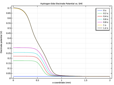
In the Settings window for 1D Plot Group, type Hydrogen-Side Electrode Potential vs. SHE in the Label text field.
Line Graph 1
1
In the Hydrogen-Side Electrode Potential vs. SHE toolbar, click  Line Graph.
2
3
In the Settings window for Line Graph, locate the y-Axis Data section.
4
In the Expression text field, type fc.Ect.
5
Locate the x-Axis Data section. From the Parameter list, choose Expression.
6
In the Expression text field, type x.
7
Click to expand the Legends section. Select the Show legends checkbox.
Hydrogen-Side Electrode Potential vs. SHE
1
In the Model Builder window, click Hydrogen-Side Electrode Potential vs. SHE.
2
In the Settings window for 1D Plot Group, click to expand the Title section.
3
From the Title type list, choose Label.
4
In the Hydrogen-Side Electrode Potential vs. SHE toolbar, click  Plot.
The plot should look like Figure 5.
Hydrogen-Side Electrode Potential vs. SHE 1
Right-click Hydrogen-Side Electrode Potential vs. SHE and choose Duplicate.
Hydrogen-Side Electrode Potential vs. SHE
In the Model Builder window, collapse the Results > Hydrogen-Side Electrode Potential vs. SHE node.
Oxygen-Side Electrode Potential vs. SHE
1
In the Model Builder window, under Results click Hydrogen-Side Electrode Potential vs. SHE 1.
2
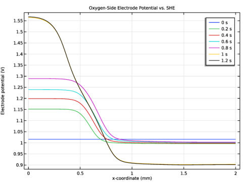
In the Settings window for 1D Plot Group, type Oxygen-Side Electrode Potential vs. SHE in the Label text field.
Line Graph 1
1
In the Model Builder window, expand the Oxygen-Side Electrode Potential vs. SHE node, then click Line Graph 1.
2
In the Settings window for Line Graph, locate the Selection section.
3
Click to select the  Activate Selection toggle button.
4
Oxygen-Side Electrode Potential vs. SHE
1
In the Model Builder window, click Oxygen-Side Electrode Potential vs. SHE.
2
In the Oxygen-Side Electrode Potential vs. SHE toolbar, click  Plot.
The plot should look like Figure 6.
Carbon Corrosion Rate in Oxygen-Side Electrode
1
Right-click Oxygen-Side Electrode Potential vs. SHE and choose Duplicate.
2
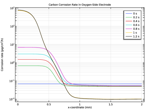
In the Settings window for 1D Plot Group, type Carbon Corrosion Rate in Oxygen-Side Electrode in the Label text field.
3
Locate the Plot Settings section.
4
Select the y-axis label checkbox. In the associated text field, type Corrosion rate (\mu g/cm<sup>2</sup>/h).
Line Graph 1
1
In the Model Builder window, expand the Carbon Corrosion Rate in Oxygen-Side Electrode node, then click Line Graph 1.
2
In the Settings window for Line Graph, locate the y-Axis Data section.
3
In the Expression text field, type CR.
4
In the Unit field, type ug/cm^2/h.
Carbon Corrosion Rate in Oxygen-Side Electrode
1
In the Model Builder window, click Carbon Corrosion Rate in Oxygen-Side Electrode.
2
In the Settings window for 1D Plot Group, locate the Axis section.
3
Select the y-axis log scale checkbox.
4
In the Carbon Corrosion Rate in Oxygen-Side Electrode toolbar, click  Plot.
The plot should look like Figure 7.
5
In the Model Builder window, collapse the Carbon Corrosion Rate in Oxygen-Side Electrode node.
Hydrogen-Side Current Density
1
In the Results toolbar, click  1D Plot Group.
2
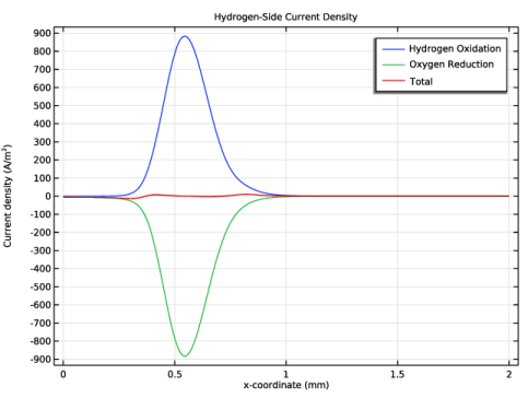
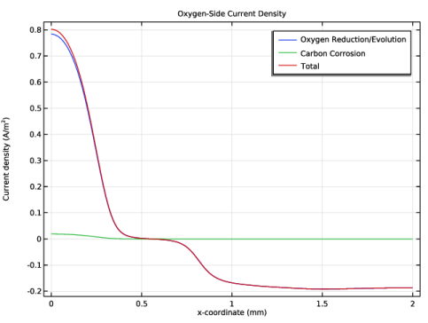
In the Settings window for 1D Plot Group, type Hydrogen-Side Current Density in the Label text field.
3
Locate the Data section. From the Time selection list, choose Last.
4
Locate the Title section. From the Title type list, choose Label.
5
Locate the Plot Settings section.
6
Select the y-axis label checkbox. In the associated text field, type Current density (A/m<sup>2</sup>).
Line Graph 1
1
In the Hydrogen-Side Current Density toolbar, click  Line Graph.
2
3
In the Settings window for Line Graph, click Replace Expression in the upper-right corner of the y-Axis Data section. From the menu, choose Component 1 (comp1) > Hydrogen Fuel Cell > Electrode kinetics > fc.iloc_th2gder1 - Local current density - A/m².
4
Locate the x-Axis Data section. From the Parameter list, choose Expression.
5
In the Expression text field, type x.
6
Locate the Legends section. Select the Show legends checkbox.
7
From the Legends list, choose Manual.
8
Line Graph 2
1
Right-click Line Graph 1 and choose Duplicate.
2
In the Settings window for Line Graph, locate the y-Axis Data section.
3
In the Expression text field, type fc.iloc_th2gder2.
4
Locate the Legends section. In the table, enter the following settings:
Line Graph 3
1
Right-click Line Graph 2 and choose Duplicate.
2
In the Settings window for Line Graph, click Replace Expression in the upper-right corner of the y-Axis Data section. From the menu, choose Component 1 (comp1) > Hydrogen Fuel Cell > Electrode kinetics > fc.itot - Total interface current density - A/m².
3
Locate the Legends section. In the table, enter the following settings:
Hydrogen-Side Current Density
1
In the Model Builder window, click Hydrogen-Side Current Density.
2
In the Hydrogen-Side Current Density toolbar, click  Plot.
The plot should look like Figure 8.
Hydrogen-Side Current Density 1
Right-click Hydrogen-Side Current Density and choose Duplicate.
Hydrogen-Side Current Density
In the Model Builder window, collapse the Results > Hydrogen-Side Current Density node.
Oxygen-Side Current Density
1
In the Model Builder window, under Results click Hydrogen-Side Current Density 1.
2
In the Settings window for 1D Plot Group, type Oxygen-Side Current Density in the Label text field.
Line Graph 1
1
In the Model Builder window, expand the Oxygen-Side Current Density node, then click Line Graph 1.
2
In the Settings window for Line Graph, locate the Selection section.
3
Click to select the  Activate Selection toggle button.
4
5
Locate the y-Axis Data section. In the Expression text field, type fc.iloc_to2gder1.
6
Locate the Legends section. In the table, enter the following settings:
Line Graph 2
1
In the Model Builder window, click Line Graph 2.
2
In the Settings window for Line Graph, locate the Selection section.
3
Click to select the  Activate Selection toggle button.
4
5
Locate the y-Axis Data section. In the Expression text field, type fc.iloc_to2gder2.
6
Locate the Legends section. In the table, enter the following settings:
Line Graph 3
1
In the Model Builder window, click Line Graph 3.
2
In the Settings window for Line Graph, locate the Selection section.
3
Click to select the  Activate Selection toggle button.
4
Oxygen-Side Current Density
1
In the Model Builder window, click Oxygen-Side Current Density.
2
In the Oxygen-Side Current Density toolbar, click  Plot.
The plot should look like Figure 9.
Follow the instructions below to improve some plot appearances and remove redundant plots.
Surface 1
1
In the Model Builder window, expand the Electrode Potential with Respect to Ground (fc) node, then click Surface 1.
2
In the Settings window for Surface, locate the Coloring and Style section.
3
From the Color table list, choose MetasepiaBlue.
Arrow Surface 1
In the Model Builder window, right-click Arrow Surface 1 and choose Disable.
Surface 1
1
In the Model Builder window, expand the Electrolyte Potential (fc) node, then click Surface 1.
2
In the Settings window for Surface, locate the Coloring and Style section.
3
From the Color table list, choose RainbowLight.
Arrow Surface 1
In the Model Builder window, right-click Arrow Surface 1 and choose Disable.
Surface 1
1
In the Model Builder window, expand the Mole Fraction, H2O (fc) node, then click Surface 1.
2
In the Settings window for Surface, locate the Coloring and Style section.
3
From the Color table list, choose Conopiformis.
Streamline 1
1
In the Model Builder window, click Streamline 1.
2
In the Settings window for Streamline, locate the Streamline Positioning section.
3
In the Density level text field, type 8.
4
Locate the Coloring and Style section. Find the Point style subsection. From the Color list, choose Cyan.
Surface 1
1
In the Model Builder window, expand the Pressure (fc) node, then click Surface 1.
2
In the Settings window for Surface, locate the Coloring and Style section.
3
From the Color table list, choose Tectocoris.
4
From the Color table type list, choose Discrete.
Streamline 1
1
In the Model Builder window, click Streamline 1.
2
In the Settings window for Streamline, locate the Streamline Positioning section.
3
In the Density level text field, type 8.
4
Locate the Coloring and Style section. Find the Point style subsection. From the Color list, choose White.
Mole Fraction, N2 (fc)
In the Model Builder window, under Results right-click Mole Fraction, N2 (fc) and choose Delete.