|
|
|
|
1
|
|
2
|
In the Select Physics tree, select Electrochemistry > Hydrogen Fuel Cells > Proton Exchange Membrane (fc).
|
|
3
|
Click Add.
|
|
4
|
|
5
|
Click Add.
|
|
6
|
Click
|
|
7
|
|
8
|
Click
|
|
1
|
|
2
|
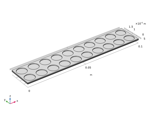
Browse to the model’s Application Libraries folder and double-click the file passive_pem_geom_sequence.mph.
|
|
3
|
|
4
|
|
1
|
|
2
|
|
1
|
|
2
|
|
1
|
|
2
|
|
1
|
|
2
|
|
1
|
|
2
|
|
3
|
|
1
|
|
2
|
|
3
|
|
1
|
|
2
|
|
3
|
|
1
|
|
2
|
|
3
|
|
1
|
|
2
|
|
3
|
|
1
|
|
2
|
|
1
|
|
2
|
|
1
|
|
2
|
|
1
|
|
2
|
|
3
|
Click
|
|
4
|
Browse to the model’s Application Libraries folder and double-click the file passive_pem_parameters.txt.
|
|
1
|
|
2
|
|
3
|
Clear the H2O checkbox.
|
|
4
|
Locate the O2 Gas Mixture section. Find the Transport mechanisms subsection. Clear the Include gas phase diffusion checkbox.
|
|
1
|
|
2
|
|
3
|
|
4
|
|
1
|
|
2
|
|
3
|
|
4
|
|
1
|
|
2
|
|
3
|
|
4
|
|
1
|
|
2
|
|
3
|
|
1
|
|
2
|
|
3
|
|
4
|
|
1
|
|
2
|
In the Settings window for Thin H2 Gas Diffusion Electrode Reaction, locate the Electrode Kinetics section.
|
|
3
|
|
4
|
|
1
|
|
2
|
|
3
|
|
4
|
|
1
|
|
2
|
In the Settings window for Thin O2 Gas Diffusion Electrode Reaction, locate the Electrode Kinetics section.
|
|
3
|
|
4
|
|
1
|
In the Model Builder window, under Component 1 (comp1) > Hydrogen Fuel Cell (fc) click O2 Gas Phase 1.
|
|
2
|
|
3
|
|
4
|
|
5
|
|
1
|
In the Model Builder window, under Component 1 (comp1) > Hydrogen Fuel Cell (fc) > Electrolyte Phase 1 click Initial Values 1.
|
|
2
|
|
3
|
|
1
|
|
2
|
|
3
|
Click
|
|
4
|
Click
|
|
5
|
|
6
|
Click OK.
|
|
7
|
|
8
|
|
1
|
|
2
|
|
3
|
|
1
|
|
2
|
|
3
|
|
4
|
|
1
|
|
1
|
|
2
|
|
3
|
|
5
|
|
6
|
|
7
|
|
1
|
|
2
|
|
3
|
|
4
|
Locate the Surface-to-Ambient Radiation section. From the ε list, choose User defined. In the associated text field, type 0.8.
|
|
5
|
|
1
|
|
3
|
In the Settings window for Surface-to-Ambient Radiation, locate the Surface-to-Ambient Radiation section.
|
|
4
|
|
5
|
|
1
|
|
2
|
Go to the Add Material window.
|
|
3
|
|
4
|
Click the Add to Component button in the window toolbar.
|
|
5
|
|
6
|
Click the Add to Component button in the window toolbar.
|
|
7
|
|
1
|
|
2
|
|
1
|
|
2
|
|
3
|
|
1
|
|
2
|
|
3
|
|
4
|
Locate the Material Contents section. In the table, enter the following settings:
|
|
5
|
|
1
|
|
2
|
|
3
|
|
4
|
Locate the Material Contents section. In the table, enter the following settings:
|
|
1
|
|
1
|
|
2
|
|
3
|
Click the Custom button.
|
|
4
|
|
5
|
|
1
|
|
2
|
|
3
|
|
4
|
|
1
|
|
2
|
|
3
|
|
1
|
|
2
|
|
3
|
|
4
|
Click
|
|
1
|
|
1
|
|
2
|
|
3
|
Click the Custom button.
|
|
4
|
Locate the Element Size Parameters section.
|
|
5
|
|
6
|
|
7
|
Click
|
|
1
|
|
2
|
|
3
|
|
1
|
|
1
|
|
2
|
In the Settings window for Boundary Probe, type Average Cell Current Density Probe in the Label text field.
|
|
3
|
|
4
|
|
5
|
Click Replace Expression in the upper-right corner of the Expression section. From the menu, choose Component 1 (comp1) > Hydrogen Fuel Cell > Electrode kinetics > fc.iloc_th2gder1 - Local current density - A/m².
|
|
6
|
|
1
|
|
2
|
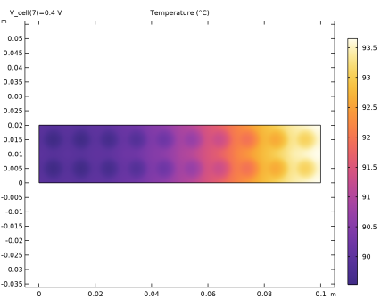
In the Settings window for Boundary Probe, type Average Cell Temperature Probe in the Label text field.
|
|
3
|
|
4
|
|
5
|
|
1
|
|
2
|
|
3
|
Select the Auxiliary sweep checkbox.
|
|
4
|
Click
|
|
1
|
|
2
|
|
3
|
|
4
|
|
5
|
In the Model Builder window, expand the Study 1 > Solver Configurations > Solution 1 (sol1) > Stationary Solver 1 > Segregated 1 node, then click Hydrogen Fuel Cell.
|
|
6
|
|
7
|
|
8
|
|
9
|
|
10
|
Clear the Generate default plots checkbox.
|
|
11
|
|
1
|
|
2
|
|
3
|
Click
|
|
4
|
|
5
|
Click OK.
|
|
6
|
|
8
|
Select the Apply conversions to expressions with the same dimensions checkbox.
|
|
9
|
|
10
|
Click
|
|
1
|
|
2
|
|
1
|
|
2
|
|
3
|
|
4
|
|
5
|
|
1
|
|
2
|
|
1
|
|
2
|
|
3
|
|
4
|
|
1
|
|
2
|
|
1
|
|
2
|
|
3
|
|
4
|
|
5
|
|
1
|
|
2
|
|
3
|
|
4
|
|
5
|
Click
|
|
1
|
|
2
|
|
1
|
|
2
|
|
3
|
|
4
|
|
5
|
|
6
|
|
1
|
|
2
|
|
1
|
|
2
|
|
3
|
|
4
|
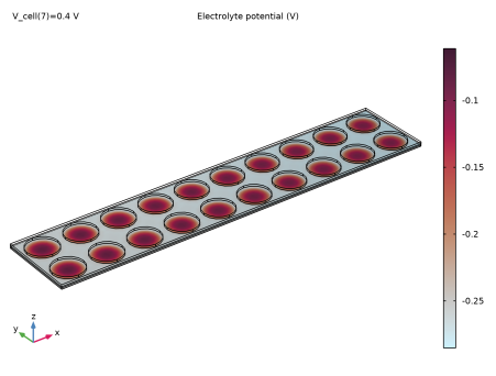
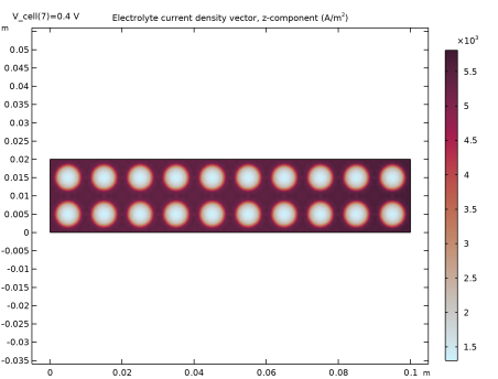
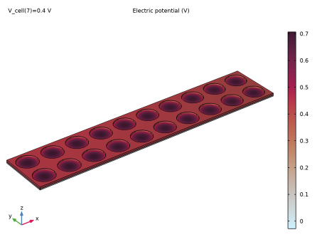
Click Replace Expression in the upper-right corner of the Expression section. From the menu, choose Component 1 (comp1) > Hydrogen Fuel Cell > Electrolyte current density vector - A/m² > fc.Ilz - Electrolyte current density vector, z-component.
|
|
5
|
|
6
|
|
1
|
|
2
|
|
3
|
Locate the Plot Settings section.
|
|
4
|
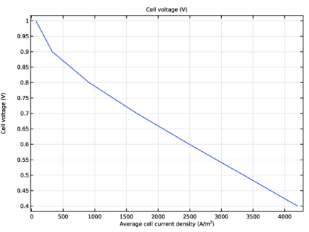
Select the x-axis label checkbox. In the associated text field, type Average cell current density (A/m<sup>2</sup>).
|
|
1
|
|
2
|
|
4
|
|
5
|
|
6
|
|
7
|
|
1
|
|
2
|
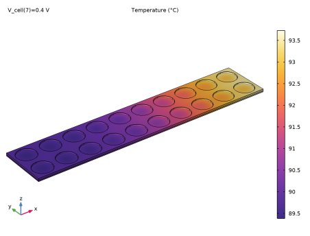
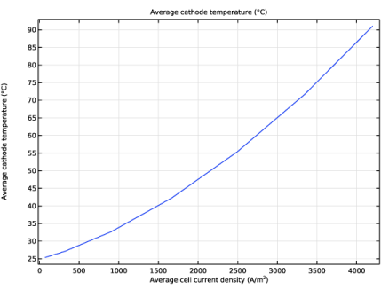
In the Settings window for 1D Plot Group, type Temperature vs. Current Density in the Label text field.
|
|
3
|
Locate the Plot Settings section.
|
|
4
|
Select the x-axis label checkbox. In the associated text field, type Average cell current density (A/m<sup>2</sup>).
|
|
1
|
|
2
|
|
4
|
|
5
|
|
6
|
|
7
|
|
1
|
|
2
|
|
1
|
|
2
|
|
3
|
|
4
|
|
5
|
|
1
|
|
2
|
|
3
|
|
4
|
|
5
|
|
6
|
|
7
|
Click
|
|
1
|
|
2
|
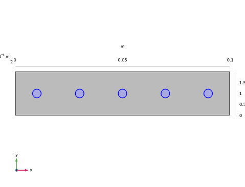
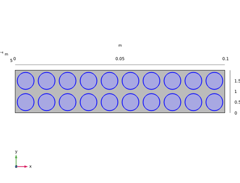
Select the object cyl1 only.
|
|
3
|
|
4
|
|
5
|
|
6
|
Click
|
|
1
|
|
2
|
|
3
|
|
4
|
|
5
|
|
6
|
Click and drag in the Graphics window to enclose and high-light all five cylinders, then right-click to confirm the selection.
 |
|
7
|
Click
|
|
8
|
|
1
|
|
2
|
|
3
|
|
4
|
|
5
|
|
6
|
|
7
|
Click
|
|
1
|
|
2
|
|
3
|
|
4
|
|
5
|
|
6
|
|
7
|
Click
|
|
1
|
|
2
|
|
3
|
|
4
|
|
5
|
|
6
|
|
7
|
Click
|
|
1
|
|
2
|
|
3
|
|
4
|
|
5
|
|
6
|
|
7
|
Click
|
|
1
|
|
2
|
|
3
|
|
4
|
|
5
|
|
6
|
|
7
|
|
8
|
Click
|
|
1
|
|
2
|
Select the object cyl2 only.
|
|
3
|
|
4
|
|
5
|
|
6
|
|
7
|
|
8
|
Click
|
|
1
|
|
2
|
|
3
|
|
4
|
|
5
|
|
6
|
Click and drag in the Graphics window to enclose and high-light the 20 cylinders, then right-click to confirm the selection.
 |
|
7
|
Click
|
|
8
|
|
1
|
|
2
|
|
3
|
|
4
|
Click
|
 .
.