PDF

Voltammetry at a Microdisk Electrode
Introduction
Cyclic voltammetry is a common electroanalytical technique. Since the 1980s, it has been common in voltammetry to use a microdisk electrode as the working electrode (Ref. 1). This is a disk electrode with a radius on the order of micrometers, embedded in an insulator whose surface is flush with the electrode.
Figure 1: Schematic of the simulation geometry for a microdisk electrode.
These very small electrodes have advantageous mass transport properties that can maximize the measured current density, and so enable the study of electrochemical behavior that would not be observable by conventional voltammetry as performed on a large macroelectrode. (See the model Cyclic Voltammetry at a Macroelectrode in 1D.)
This example demonstrates the use of a common approximation in which an electrode with microscale dimensions is assumed to have stationary (equilibrium) diffusion properties on the time scale of a voltammetry study. This simplifies the analysis because a time-dependent model is not required. Instead, a Parametric Sweep is used to assemble a voltammogram under a quasistatic approximation.
Model Definition
The model contains a 2D axisymmetric domain surrounded by a concentric region in which Infinite Elements are used to extend the bulk solution in the model to ‘infinity’. The approximation that the bulk solution is infinitely distant is suitable if the electrochemical cell is several orders of magnitude larger than the electrode.
The x-axis is divided by a point at the electrode radius, re, which equals 10 μm. At r < re, this axis represents the working electrode (microdisk) where the electrochemical reaction takes place. At r > re, this axis represents the surrounding insulator in-plane with the disk electrode.
DOMAIN EQUATIONS
We assume the presence of a large quantity of supporting electrolyte. This is inert salt that is added in electroanalytical experiments to increase the conductivity of the electrolyte without otherwise interfering with the reaction chemistry. Under these conditions, the resistance of the solution is sufficiently low that the electric field is negligible, and we can assume that the electrolyte potential ϕl = 0 (Ref. 2).
The Electroanalysis interface implements chemical species transport equations for the reactant and product species of the redox couple subject to this assumption. The domain equation is the diffusion equation (also known as Fick’s 2nd law), which describes the chemical transport of the electroactive species A and B. At steady-state, this reduces to:
Here Di represents the diffusion coefficient and ci the concentration of a species.
BOUNDARY EQUATIONS
At the bulk boundary (r → ∞), we assume a uniform concentration equal to the bulk concentration for the reactant. The product has zero concentration here, as in bulk.
At the insulating (inert) surface, the normal flux of both species A and B equals zero, since this surface is impermeable and neither species reacts there.
At the electrode boundary, the reactant species A oxidizes (loses one electron) to form the product B. By convention, electrochemical reactions are written in the reductive direction:
The stoichiometric coefficient is –1 for B, the “reactant” in the reductive direction, and +1 for A, the “product” in the reductive direction. This formulation is consistent even in examples such as this model where at certain applied potentials, the reaction proceeds favorably to convert A to B. The number of electrons transferred, n, equals one.
The current density for this reaction is given by the electroanalytical Butler–Volmer equation for an oxidation:
in which iloc is the local current density, k0 is the heterogeneous rate constant of the reaction, αc is the cathodic transfer coefficient, and η is the overpotential at the working electrode. Additionally, F, R, T, represent Faraday’s constant, the ideal gas constant and the temperature, respectively.
According to Faraday’s laws of electrolysis, the flux of the reactant and product species are proportional to the current density drawn:
Here n is the normal vector of the boundary, Ji the molar flux, and the product -n · Ji the molar flux across the boundary. Additionally, νi represents the stoichiometric factor and n the number of electrons transferred.
This is expressed in the Electrode Surface boundary condition.
The total current, Iel, recorded at the disk electrode can be extracted by integrating the local current density across the electrode surface. For this purpose, the Electroanalysis interface defines an electrode current variable according to
Note that it is not sufficient to simply multiply by the area of the electrode, because the current density may be nonuniform.
STATIONARY STUDY
In contrast to macroelectrode voltammetry, a voltammogram recorded at a microdisk does not exhibit hysteresis. Diffusion is so fast on the time scale of the experiment that a stationary approximation is suitable. A quasistatic approximation applies when:
where v is the voltammetric scan rate (SI unit: V/s). The two terms in this inequality are respectively the diffusive and voltammetric time scales of the system.
Within the Stationary study, a parametric sweep is used to study the range of applied potentials achieved in the voltammogram.
Results and Discussion
The stationary concentration profile around a microdisk electrode (Figure 2) has a distinct shape. At large distances from the electrode, the concentration profile is roughly hemispherical, but close to the disk edge the flux is elevated. For fast kinetics the concentrations on the electrode surface are roughly equilibrated and so are uniform. This leads to unequal flux over the surface of the electrode — it is nonuniformly accessible.
Figure 2: Characteristic concentration profile and mass flux streamlines for transport-controlled oxidation of species A at a microdisk electrode (2D cross section).
The shape of the cyclic voltammogram (Figure 3) illustrates the relation between electrode kinetics and chemical species transport (diffusion).
Figure 3: Quasistatic (steady-state) cyclic voltammetry recorded at a microdisk electrode. We can here see the limiting current density as explained below.
Initially, at reducing potentials, the oxidation reaction is not driven, and negligible current is drawn. As the potential moves toward the reduction potential of the redox couple (0 V), the oxidation reaction is accelerated and the current increases.
Once the oxidation reaction is fast enough that it consumes significant reactant at the electrode surface, the current becomes limited by the rate of transport of A toward the working electrode. Because the diffusion layer is equilibrated, this transport-limited current is constant in time and independent of applied potential. The analytical Saito equation gives this limiting current as (Ref. 3):
where c is the bulk concentration of reactant.
Negative current is never observed for the “steady-state” voltammetry at a microdisk electrode, since the product species is effectively dispersed to bulk solution. Rapid diffusion on the voltammetric time scale ensures equilibration between the bulk and the electrode surface. Because of the absence of product in bulk, this equilibrium means that the reaction is always oxidative.
Notes About the COMSOL Implementation
A refined mesh is required close to the electrode surface in order to accurately resolve the concentration profile, and hence the current. The mesh is refined further close to the singularity where the electrode and insulator boundaries meet. In the Infinite Element Domain, a Swept mesh is used.
Figure 4: Customized mesh used for the microdisk analysis.
References
1. R.G. Compton and C.E. Banks, Understanding Voltammetry, 2nd ed., London, 2011.
2. A.J. Bard and L.R. Faulkner, Electrochemical Methods, Fundamentals and Applications, 2nd ed., Hoboken, 2001.
3. Y. Saito, Review of Polarography (Japan), vol. 15, pp. 177–187, 1968.
Application Library path: Fuel_Cell_and_Electrolyzer_Module/General_Electrochemistry/microdisk_voltammetry
Modeling Instructions
From the File menu, choose New.
New
In the New window, click  Model Wizard.
Model Wizard
1
In the Model Wizard window, click  2D Axisymmetric.
2
In the Select Physics tree, select Electrochemistry > Electroanalysis (tcd).
3
Click Add.
4
In the Concentrations (mol/m³) table, enter the following settings:
5
Click  Study.
6
In the Select Study tree, select General Studies > Stationary.
7
Global Definitions
Load the model parameters from a text file.
Parameters 1
1
In the Model Builder window, under Global Definitions click Parameters 1.
2
In the Settings window for Parameters, locate the Parameters section.
3
Click  Load from File.
4
Geometry 1
Draw the model geometry as a quarter circle, and specify the electrode disk radius using a point as follows:
Circle 1 (c1)
1
In the Geometry toolbar, click  Circle.
2
In the Settings window for Circle, locate the Size and Shape section.
3
In the Radius text field, type r_max.
4
In the Sector angle text field, type 90.
Point 1 (pt1)
1
In the Geometry toolbar, click  Point.
2
In the Settings window for Point, locate the Point section.
3
In the r text field, type re.
Circle 1 (c1)
Add a second circle that will be used to set up an Infinite Element domain as follows:
Circle 2 (c2)
1
In the Model Builder window, under Component 1 (comp1) > Geometry 1 right-click Circle 1 (c1) and choose Duplicate.
2
In the Settings window for Circle, locate the Size and Shape section.
3
In the Radius text field, type r_max*1.2.
4
In the Geometry toolbar, click  Build All.
5
Click the  Zoom Extents button in the Graphics toolbar.
Your finalized geometry should now like this:
6
In the Model Builder window, click Geometry 1.
Definitions
Add an Infinite Element domain, and assign it to the outer domain.
Infinite Element Domain 1 (ie1)
1
In the Definitions toolbar, click  Infinite Element Domain.
You can select an element by clicking on it in the graphics window.
2
Electroanalysis (tcd)
Electrolyte 1
Now start setting up the physics. Start with the diffusion coefficients.
1
In the Model Builder window, under Component 1 (comp1) > Electroanalysis (tcd) click Electrolyte 1.
2
In the Settings window for Electrolyte, locate the Diffusion section.
3
In the DcRed text field, type D1.
4
In the DcOx text field, type D2.
Electrode Surface 1
Add an Electrode Surface boundary node. Set up the electrode kinetics in the Electrode Reaction subnode as follows:
1
In the Physics toolbar, click  Boundaries and choose Electrode Surface.
2
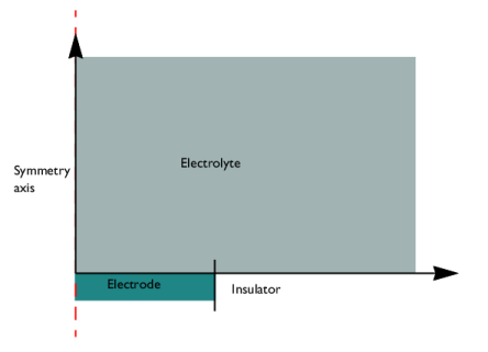
In the Settings window for Electrode Surface, locate the Electrode Phase Potential Condition section.
3
From the Electrode phase potential condition list, choose Electrode potential.
4
In the Evsref text field, type E_appl.
5
Electrode Reaction 1
1
In the Model Builder window, click Electrode Reaction 1.
2
In the Settings window for Electrode Reaction, locate the Stoichiometric Coefficients section.
3
In the νcRed text field, type 1.
4
In the νcOx text field, type -1.
5
Locate the Equilibrium Potential section. In the Eeq,ref(T) text field, type Ef.
6
Locate the Electrode Kinetics section. In the i0,ref(T) text field, type i0ref.
Concentration 1
Specify the bulk composition at the outer boundary.
1
In the Physics toolbar, click  Boundaries and choose Concentration.
2
3
In the Settings window for Concentration, locate the Concentration section.
4
Select the Species cRed checkbox.
5
In the c0,cRed text field, type c_bulk.
6
Select the Species cOx checkbox.
Initial Values 1
1
In the Model Builder window, click Initial Values 1.
2
In the Settings window for Initial Values, locate the Initial Values section.
3
In the cRed text field, type c_bulk.
Mesh 1
Edit the default mesh to ensure good numerical accuracy.
1
In the Model Builder window, under Component 1 (comp1) right-click Mesh 1 and choose Edit Physics-Induced Sequence.
Size
1
In the Model Builder window, under Component 1 (comp1) > Mesh 1 click Size.
2
In the Settings window for Size, locate the Element Size section.
3
From the Predefined list, choose Finer.
4
Click to expand the Element Size Parameters section. In the Maximum element growth rate text field, type 1.1.
Free Triangular 1
1
In the Model Builder window, click Free Triangular 1.
2
In the Settings window for Free Triangular, locate the Domain Selection section.
3
From the Geometric entity level list, choose Domain.
4
Size 1
1
Right-click Free Triangular 1 and choose Size.
2
In the Settings window for Size, locate the Geometric Entity Selection section.
3
From the Geometric entity level list, choose Point.
4
5
Locate the Element Size section. Click the Custom button.
6
Locate the Element Size Parameters section.
7
Select the Maximum element size checkbox. In the associated text field, type re/100.
Mapped 1
1
In the Mesh toolbar, click  Mapped.
2
In the Settings window for Mapped, locate the Domain Selection section.
3
From the Geometric entity level list, choose Domain.
4
5
In the Model Builder window, right-click Mesh 1 and choose Build All.
Study 1
The problem is now ready for solving. Simulate a voltammogram by using a Parametric Sweep for a range of applied potentials.
Parametric Sweep
1
In the Study toolbar, click  Parametric Sweep.
2
In the Settings window for Parametric Sweep, locate the Study Settings section.
3
4
5
In the Study toolbar, click  Compute.
Results
Concentration, Red (tcd)
Two concentration plots are created by default for each species: one in 2D and one revolved 3D plot.
Modify the first default plot as follows:
Definitions
Change the default 2D view to show the results more clearly. Start by changing the view for the model and its plot. We want to position the view close to the electrode surface.
Axis
1
In the Model Builder window, expand the Component 1 (comp1) > Definitions > View 1 node, then click Axis.
2
In the Settings window for Axis, locate the Axis section.
3
In the r minimum text field, type -1e-6.
4
In the r maximum text field, type 1e-4.
5
In the z minimum text field, type -5e-7.
6
In the z maximum text field, type 1e-4.
7
Click  Update.
Results
Concentration, Red (tcd)
1
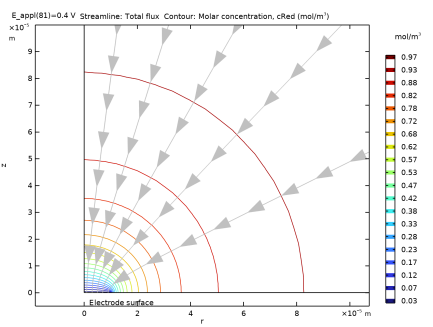
In the Model Builder window, expand the Results > Concentration, Red (tcd) node, then click Concentration, Red (tcd).
2
In the Settings window for 2D Plot Group, locate the Plot Settings section.
3
Select the x-axis label checkbox. In the associated text field, type r.
4
Select the y-axis label checkbox. In the associated text field, type z.
5
Locate the Color Legend section. Select the Show units checkbox.
Surface 1
Next, replace the surface plot with a contour plot for the concentration. Keep the streamlines for the total flux that show the increased reaction rate at the electrode edge compared with the center of the electrode.
In the Model Builder window, right-click Surface 1 and choose Disable.
Contour 1
1
In the Model Builder window, right-click Concentration, Red (tcd) and choose Contour.
2
In the Settings window for Contour, locate the Expression section.
3
In the Expression text field, type cRed.
4
Locate the Coloring and Style section. From the Contour type list, choose Tube.
5
Select the Radius scale factor checkbox. In the associated text field, type 1.2E-7.
Streamline 1
Polish the default streamline plot a little.
1
In the Model Builder window, click Streamline 1.
2
In the Settings window for Streamline, locate the Streamline Positioning section.
3
From the Positioning list, choose On selected boundaries.
4
In the Number text field, type 5.
5
Locate the Selection section. Click to select the  Activate Selection toggle button.
6
7
Locate the Coloring and Style section. Find the Point style subsection. From the Arrow length list, choose Normalized.
8
Select the Number of arrows checkbox. In the associated text field, type 100.
Annotation 1
1
In the Model Builder window, right-click Concentration, Red (tcd) and choose Annotation.
2
In the Settings window for Annotation, locate the Annotation section.
3
In the Text text field, type Electrode surface.
4
Locate the Position section. In the Z text field, type -1.5e-6.
5
Locate the Coloring and Style section. Clear the Show point checkbox.
Total current
Create a plot of the voltammogram as follows:
1
In the Home toolbar, click  Add Plot Group and choose 1D Plot Group.
2
In the Settings window for 1D Plot Group, type Total current in the Label text field.
3
Locate the Legend section. Clear the Show legends checkbox.
4
Click to expand the Title section. From the Title type list, choose None.
Global 1
1
Right-click Total current and choose Global.
2
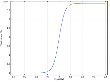
In the Settings window for Global, click Replace Expression in the upper-right corner of the y-Axis Data section. From the menu, choose Component 1 (comp1) > Electroanalysis > Electrode kinetics > tcd.Itot_es1 - Total current - A.
3
In the Total current toolbar, click  Plot.