

PDF

Liquid Alkaline Electrolyzer with Concentrated Electrolyte Transport
Introduction
This tutorial demonstrates how to modify a concentration-independent (also known as a secondary current distribution) liquid alkaline water electrolyzer with concentrated electrolyte theory to explicitly resolve local electrolyte and solvent concentrations (thereby creating a tertiary current distribution). A liquid alkaline electrolyzer is defined in a 2D model with a separator, two gas–electrolyte compartments, and negative hydrogen and positive oxygen electrodes at the boundaries. A stationary solver is used with the cell voltage swept over a range of potentials to generate a polarization curve.
The model is first solved for a secondary current distribution only. Concentrated electrolyte theory is then taken into account and the cell performance is compared between the secondary and tertiary current distribution cases.
Model Definition
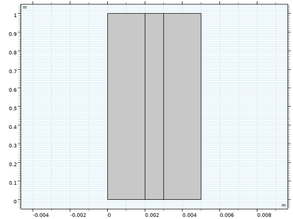
The model geometry can be seen in Figure 1.
Figure 1: Alkaline electrolyzer geometry. The x-axis is scaled by a factor of 100.
The geometry is identical to that found in the Alkaline Electrolyzer tutorial model. The geometry in Figure 1 and all subsequent figures is scaled on the x-axis by a factor of 100. In brief, two electrolyte compartments are placed on either side of an ion-conducting porous separator, with the entire system permeated by 6M KOH. Liquid flows in from the bottom of the electrolyzer and exits the top. The electrodes are located on left and right exterior walls of the electrolyte compartments.
In the standard case, the Water Electrolyzer interface is used in a secondary current distribution formulation to capture the behavior of the system. Butler–Volmer kinetics is used at both electrodes to describe the reaction rates, with the following reactions:
(1)
(2)
Reaction 1 is hydrogen evolution (reduction) and occurs at the cathode (left electrode). Reaction 2 is oxygen evolution (oxidation) and occurs at the anode (right electrode). The electrodes are considered to be flat plates (not porous electrodes).
When using a secondary current distribution, electrolyte charge transport is computed using Ohm’s law, assuming a constant conductivity and neglecting gradients in species concentration. In the second and main case examined here, this assumption is replaced with a more strict calculation of the ion and solvent concentrations everywhere in the electrolyte using the Maxwell–Stefan–Onsager theory of concentrated electrolyte transport. This behavior is captured by the Concentrated Electrolyte Transport interface.
To describe species transport using the CET interface, it is necessary to know the binary diffusion coefficients for each species pair (potassium–water, hydroxide–water, and potassium–hydroxide). These are typically determined by experimental measurements.
For a binary electrolyte in a single solvent, the three parameters conductivity, transport number of the positive ion, and salt diffusivity may be used to determine the three required binary diffusion coefficients. The three diffusion coefficients are calculated as follows:
(3)
(4)
(5)
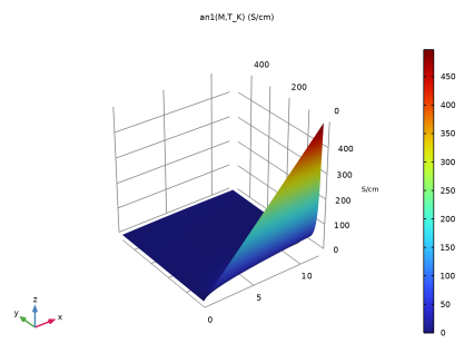
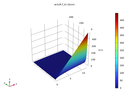
where F is Faraday’s constant (C/mol), T is the temperature (K), ci is the concentration of species i (mol/m3), cT is the total concentration (mol/m3), Di,j is the binary diffusion coefficient (m2/s), DKOH is the KOH diffusivity in water (m2/s), tK is the transport number of potassium, and κ is the conductivity (S/m). The conductivity is determined as a function of concentration and temperature from an analytical expression based on experimental data. A plot of the conductivity can be seen in Figure 2.
Figure 2: Conductivity of potassium hydroxide as a function of concentration (x-axis, M) and temperature (y-axis, °C).
In the Free and Porous Media Flow interface, laminar flow in the electrolyte compartments is combined with porous media flow in the separator. This fluid flow is coupled to the CET interface by using the density as computed by CET as the fluid density and setting the velocity field in CET to that of the Free and Porous Media Flow computed field. Flow at the electrodes due to electrochemical reaction is defined by the current at the electrode and Faraday’s Law.
Results and Discussion
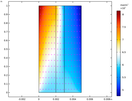
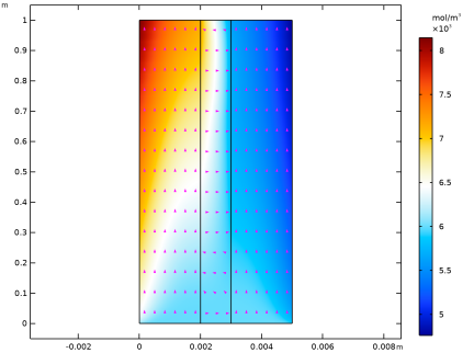
Figure 3: Concentration profile (surface) and total flux direction (arrow surface) of potassium ion.
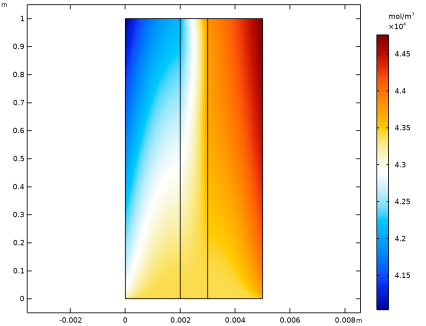
The concentration of potassium ion in the electrolyzer in the CET case can be seen in Figure 3. The concentration is higher near the outlet of the electrolyzer as well as near the cathode, where hydroxide ions are produced. Electroneutrality requires that the potassium concentration increases with the hydroxide concentration.
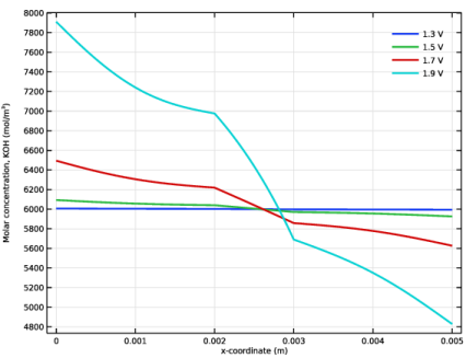
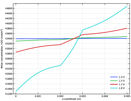
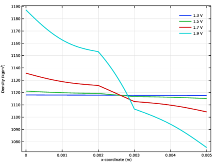
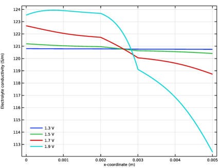
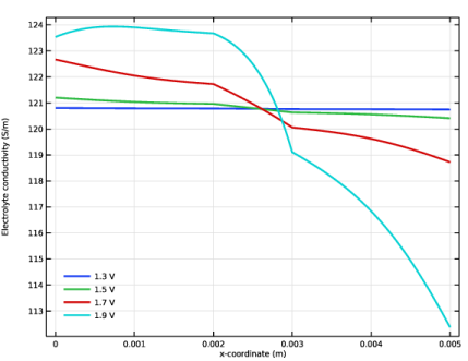
Figure 4 shows how the conductivity in the electrolyzer changes with applied voltage (and therefore concentration). As the voltage increases, conductivity increases in areas of higher concentration and decreases in areas of lower concentration.
Figure 4: Electrolyte conductivity as a function of x at y = 0.85 m.
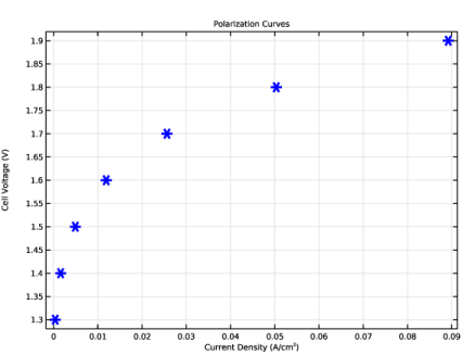
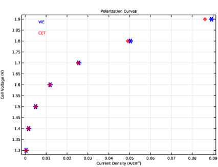
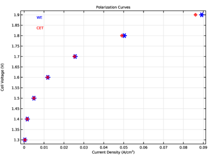
Figure 5 demonstrates the difference between the polarization curves calculated in the WE case and the CET case. The difference in conductivity caused by the concentration gradients in the CET case results in slightly more resistance and lower current density at the same voltage compared to when the system is solved without considering concentration gradients.
Figure 5: Comparison of polarization curves between the WE (blue star) and CET (red diamond) cases.
Reference
1. J. Newman and K.E. Thomas-Alyea, Electrochemical Systems, 3rd Ed. John Wiley & Sons, Hoboken, NJ, 2004.
Application Library path: Fuel_Cell_and_Electrolyzer_Module/Electrolyzers/aec_concentrated_electrolyte
Modeling Instructions
This tutorial is in two parts. First, a polarization curve for a standard liquid alkaline water electrolyzer is generated using the Water Electrolyzer interface only. Then, the Concentrated Electrolyte Transport and Free and Porous Media Flow, Brinkman interfaces are activated, the concentration and velocity profiles are examined, and the new polarization curve is compared with the initial polarization curve.
From the File menu, choose New.
New
In the New window, click  Model Wizard.
Model Wizard
1
In the Model Wizard window, click  2D.
2
In the Select Physics tree, select Electrochemistry > Water Electrolyzers > Alkaline (we).
3
Click Add.
4
Click  Study.
5
In the Select Study tree, select Preset Studies for Selected Physics Interfaces > Stationary with Initialization.
6
Global Definitions
Load model parameters from a text file.
Parameters 1
1
In the Model Builder window, under Global Definitions click Parameters 1.
2
In the Settings window for Parameters, locate the Parameters section.
3
Click  Load from File.
4
Geometry 1
The basic geometry is the same as that used in Alkaline Electrolyzer, so it is imported here. The height parameter is then modified for this model. Since the aspect ratio of the geometry is large define a View that scales the x-axis 100 times.
1
In the Geometry toolbar, click Insert Sequence and choose Insert Sequence.
2
Global Definitions
1
In the Model Builder window, under Global Definitions click Parameters 1.
2
In the Settings window for Parameters, locate the Parameters section.
3
Geometry 1
1
In the Geometry toolbar, click  Build All.
2
In the Model Builder window, under Component 1 (comp1) click Geometry 1.
Since the aspect ratio of the geometry is large define a View that scales the x-axis 100 times.
Definitions
View 2
1
In the Model Builder window, expand the Component 1 (comp1) > Definitions node.
2
Right-click Definitions and choose View.
Axis
1
In the Model Builder window, expand the View 2 node, then click Axis.
2
In the Settings window for Axis, locate the Axis section.
3
From the View scale list, choose Manual.
4
In the x scale text field, type 100.
5
Click  Update.
6
Click the  Zoom Extents button in the Graphics toolbar.
Variables - Electrodes
Load local variables from a text file. Note that the Electrodes variables are only active on the electrode boundaries.
1
In the Home toolbar, click  Variables and choose Local Variables.
2
In the Settings window for Definitions, in the Graphics window toolbar, clicknext to  Go to Default View, then choose Go to View 2.
3
In the Model Builder window, click Variables 1.
4
In the Settings window for Variables, locate the Variables section.
5
Click  Load from File.
6
Browse to the model’s Application Libraries folder and double-click the file aec_concentrated_electrolyte_variables_electrode.txt.
7
Locate the Geometric Entity Selection section. From the Geometric entity level list, choose Boundary.
8
From the Selection list, choose Electrodes.
9
In the Label text field, type Variables - Electrodes.
Electrode Average
Define an averaging function on the oxygen electrode to use for determining the cell current density for the polarization curves in both studies.
1
In the Definitions toolbar, click  Nonlocal Couplings and choose Average.
2
In the Settings window for Average, type Electrode Average in the Label text field.
3
Locate the Source Selection section. From the Geometric entity level list, choose Boundary.
4
From the Selection list, choose Oxygen Electrode.
Materials
Add the electrolyte material for KOH here. The electrolyte conductivity varies with the dimensionless concentration and temperature, as shown in the plot.
Add Material
1
In the Materials toolbar, click  Add Material to open the Add Material window.
2
Go to the Add Material window.
3
In the tree, select Fuel Cell and Electrolyzer > Aqueous Alkali > Potassium Hydroxide, KOH.
4
Click the right end of the Add to Global Materials split button in the window toolbar.
5
From the menu, choose Add to Component.
6
In the Materials toolbar, click  Add Material to close the Add Material window.
Materials
Potassium Hydroxide, KOH (mat1)
In the Model Builder window, expand the Component 1 (comp1) > Materials > Potassium Hydroxide, KOH (mat1) node.
Analytic 1 (an1)
1
In the Model Builder window, expand the Component 1 (comp1) > Materials > Potassium Hydroxide, KOH (mat1) > Electrolyte conductivity (ionc) node, then click Analytic 1 (an1).
2
In the Settings window for Analytic, click  Plot.
Global Definitions
Default Model Inputs
1
In the Model Builder window, under Global Definitions click Default Model Inputs.
2
In the Settings window for Default Model Inputs, locate the Browse Model Inputs section.
3
In the tree, select General > Temperature (K) - minput.T.
4
Find the Expression for remaining selection subsection. In the Temperature text field, type T.
5
In the tree, select General > Concentration (mol/m^3) - minput.c.
6
In the Concentration text field, type c.
Water Electrolyzer (we)
Now, the Water Electrolyzer interface can be set up for the first case, without using CET and Fluid Flow. Note that gas-phase diffusion in the electrolyte is not considered here.
1
In the Model Builder window, under Component 1 (comp1) click Water Electrolyzer (we).
2
In the Settings window for Water Electrolyzer, locate the H2 Gas Mixture section.
3
Find the Transport mechanisms subsection. Clear the Include gas phase diffusion checkbox.
4
Locate the O2 Gas Mixture section. Clear the Include gas phase diffusion checkbox.
H2 Gas Phase 1
1
In the Model Builder window, under Component 1 (comp1) > Water Electrolyzer (we) click H2 Gas Phase 1.
2
In the Settings window for H2 Gas Phase, locate the Composition section.
3
From the Mixture specification list, choose Humidified mixture.
4
In the Thum text field, type T.
O2 Gas Phase 1
1
In the Model Builder window, click O2 Gas Phase 1.
2
In the Settings window for O2 Gas Phase, locate the Composition section.
3
From the Mixture specification list, choose Humidified mixture.
4
In the Thum text field, type T.
H2 Gas-Electrolyte Compartment 1
1
In the Physics toolbar, click  Domains and choose H2 Gas-Electrolyte Compartment.
2
In the Settings window for H2 Gas-Electrolyte Compartment, locate the Domain Selection section.
3
From the Selection list, choose Hydrogen Gas Compartment.
O2 Gas-Electrolyte Compartment 1
1
In the Physics toolbar, click  Domains and choose O2 Gas-Electrolyte Compartment.
2
In the Settings window for O2 Gas-Electrolyte Compartment, locate the Domain Selection section.
3
From the Selection list, choose Oxygen Gas Compartment.
Separator 1
1
In the Physics toolbar, click  Domains and choose Separator.
2
In the Settings window for Separator, locate the Domain Selection section.
3
From the Selection list, choose Separator.
4
Locate the Effective Electrolyte Charge Transport section. In the εl text field, type eps_sep.
H2 Electrode Surface 1
1
In the Physics toolbar, click  Boundaries and choose H2 Electrode Surface.
2
In the Settings window for H2 Electrode Surface, locate the Boundary Selection section.
3
From the Selection list, choose Hydrogen Electrode.
H2 Electrode Reaction 1
1
In the Model Builder window, click H2 Electrode Reaction 1.
2
In the Settings window for H2 Electrode Reaction, locate the Electrode Kinetics section.
3
In the i0,ref(T) text field, type i0_ref_H2*i0_f_H2.
4
Locate the Stoichiometric Coefficients section. In the νH2O text field, type 0.
5
In the νH2O(l) text field, type -1.
O2 Electrode Surface 1
1
In the Physics toolbar, click  Boundaries and choose O2 Electrode Surface.
2
In the Settings window for O2 Electrode Surface, locate the Boundary Selection section.
3
From the Selection list, choose Oxygen Electrode.
4
Locate the Electrode Phase Potential Condition section. In the ϕs,ext text field, type E_cell.
O2 Electrode Reaction 1
1
In the Model Builder window, click O2 Electrode Reaction 1.
2
In the Settings window for O2 Electrode Reaction, locate the Electrode Kinetics section.
3
In the i0,ref(T) text field, type i0_ref_O2*i0_f_O2.
4
Locate the Stoichiometric Coefficients section. In the νH2O(l) text field, type -1.
5
In the νH2O text field, type 0.
Mesh 1
To ensure that the flows near the domain boundaries are accurately resolved, refine the mesh near the electrode and separator surfaces using the Boundary Layer mesh functionality. This improves convergence in the second part of the study. Set up the meshing sequence manually as follows:
Mapped 1
In the Mesh toolbar, click  Mapped.
Size
1
In the Model Builder window, click Size.
2
In the Settings window for Size, locate the Element Size section.
3
From the Predefined list, choose Finer.
4
Click to expand the Element Size Parameters section.
Distribution 1
1
In the Mesh toolbar, click  Distribution.
2
In the Settings window for Distribution, locate the Distribution section.
3
In the Number of elements text field, type 8.
4
Boundary Layers 1
1
In the Mesh toolbar, click  Boundary Layers.
2
In the Settings window for Boundary Layers, locate the Domain Selection section.
3
From the Geometric entity level list, choose Domain.
4
From the Selection list, choose Gas Compartments.
5
Click to expand the Transition section. Clear the Smooth transition to interior mesh checkbox.
Boundary Layer Properties
1
In the Model Builder window, click Boundary Layer Properties.
2
3
In the Settings window for Boundary Layer Properties, locate the Layers section.
4
In the Number of layers text field, type 3.
Study 1 - WE Only
1
In the Model Builder window, click Study 1.
2
In the Settings window for Study, type Study 1 - WE Only in the Label text field.
Step 2: Stationary
1
In the Model Builder window, under Study 1 - WE Only click Step 2: Stationary.
2
In the Settings window for Stationary, click to expand the Study Extensions section.
3
Select the Auxiliary sweep checkbox.
4
5
6
In the Study toolbar, click  Compute.
Results
Polarization Curves
Plot the polarization curve for the WE model to confirm that the system solved appropriately.
1
In the Results toolbar, click  1D Plot Group.
2
In the Settings window for 1D Plot Group, click to expand the Title section.
3
From the Title type list, choose Manual.
4
In the Title text area, type Polarization Curve.
5
Locate the Plot Settings section.
6
Select the x-axis label checkbox. In the associated text field, type Current Density (A/cm<sup>2</sup>).
7
Locate the Title section. In the Title text area, type Polarization Curves.
8
In the Label text field, type Polarization Curves.
Line Graph 1
1
In the Polarization Curves toolbar, click  Line Graph.
2
3
In the Settings window for Line Graph, locate the y-Axis Data section.
4
In the Expression text field, type E_cell.
5
Locate the x-Axis Data section. From the Parameter list, choose Expression.
6
In the Expression text field, type aveop1(we.itot).
7
In the Unit field, type A/cm^2.
8
Click to expand the Coloring and Style section. Locate the Data section. From the Dataset list, choose Study 1 - WE Only/Solution 1 (sol1).
9
Locate the Coloring and Style section. From the Color list, choose Blue.
10
From the Width list, choose 2.
11
Find the Line markers subsection. From the Marker list, choose Asterisk.
12
In the Polarization Curves toolbar, click  Plot.
Add Physics
Now add the appropriate physics to solve the system with CET.
1
In the Home toolbar, click  Add Physics to open the Add Physics window.
2
Go to the Add Physics window.
3
In the tree, select Electrochemistry > Concentrated Electrolyte Transport (cet).
4
Click the Add to Component 1 button in the window toolbar.
5
In the tree, select Fluid Flow > Porous Media and Subsurface Flow > Free and Porous Media Flow, Brinkman (fp).
6
Click the Add to Component 1 button in the window toolbar.
7
In the Home toolbar, click  Add Physics to close the Add Physics window.
Definitions
Additional variables and the inlet velocity profile must be added for the CET model.
Variables - KOH Properties, CET
1
In the Home toolbar, click  Variables and choose Local Variables.
2
In the Settings window for Variables, locate the Variables section.
3
Click  Load from File.
4
5
In the Label text field, type Variables - KOH Properties, CET.
Inlet Velocity Profile
1
In the Home toolbar, click  Functions and choose Local > Piecewise.
2
In the Settings window for Piecewise, type Inlet Velocity Profile in the Label text field.
3
Locate the Definition section. Find the Intervals subsection. Click  Load from File.
4
5
Locate the Units section. In the Arguments text field, type m.
6
In the Function text field, type m/s.
Water Electrolyzer (we)
To properly couple the CET interface to the Water Electrolyzer interface, Solve for electrolyte phase potential must be cleared and cet.phil used as the electrolyte potential variable in the Water Electrolyzer interface.
1
In the Model Builder window, under Component 1 (comp1) click Water Electrolyzer (we).
2
In the Settings window for Water Electrolyzer, click to expand the Electrolyte and Membrane Transport section.
3
Find the Electrolyte transport subsection. Clear the Solve for electrolyte phase potential checkbox.
Electrolyte Phase 1
1
In the Model Builder window, under Component 1 (comp1) > Water Electrolyzer (we) click Electrolyte Phase 1.
2
In the Settings window for Electrolyte Phase, locate the Electrolyte Phase Potential section.
3
In the ϕl text field, type cet.phil.
Concentrated Electrolyte Transport (cet)
The Concentrated Electrolyte Transport interface can now be used with KOH as the dissolved species and water as the solvent.
1
In the Model Builder window, under Component 1 (comp1) click Concentrated Electrolyte Transport (cet).
2
In the Settings window for Concentrated Electrolyte Transport, locate the Species section.
3
Find the Cations subsection. In the table, enter the following settings:
4
Find the Anions subsection. In the table, enter the following settings:
5
Find the Neutral species subsection. In the table, enter the following settings:
Reference Electrode 1
Hydrogen evolution is used as the reference reaction here.
1
In the Model Builder window, under Component 1 (comp1) > Concentrated Electrolyte Transport (cet) click Reference Electrode 1.
2
In the Settings window for Reference Electrode, locate the Stoichiometric Coefficients section.
3
In the sK text field, type 0.
4
In the sOH text field, type 1.
5
In the sH2O text field, type -1.
Electrolyte 1
1
In the Model Builder window, click Electrolyte 1.
2
In the Settings window for Electrolyte, locate the Model Input section.
3
From the T list, choose User defined. In the associated text field, type T.
4
Locate the Convection section. From the u list, choose Velocity field (fp). In the corresponding text fields, type V_KOH for potassium hydroxide and V_w for water, respectively.
Diffusion Coefficients 1
The binary diffusion coefficients are defined in the variables imported in an earlier step. The values are calculated from the conductivity, diffusion coefficient, and transport number; see the Model Definition section.
1
In the Model Builder window, click Diffusion Coefficients 1.
2
In the Settings window for Diffusion Coefficients, locate the Maxwell–Stefan Diffusivities section.
3
In the DK,OH text field, type D_K_OH.
4
In the DK,H2O text field, type D_K_H2O.
5
In the DOH,H2O text field, type D_OH_H2O.
Initial Values 1
. In the corresponding text field, type c.
Separator 1
1
In the Physics toolbar, click  Domains and choose Separator.
2
In the Settings window for Separator, locate the Domain Selection section.
3
From the Selection list, choose Separator.
4
Locate the Separator section. In the εl text field, type eps_sep.
Flow Out
1
In the Physics toolbar, click  Boundaries and choose Outflow.
2
In the Settings window for Outflow, locate the Boundary Selection section.
3
From the Selection list, choose Outlets.
4
In the Label text field, type Flow Out.
Flow In
1
In the Physics toolbar, click  Boundaries and choose Inflow.
2
In the Settings window for Inflow, locate the Inflow section.
3
From the Boundary condition type list, choose Flux (Danckwerts).
4
Locate the Boundary Selection section. From the Selection list, choose Inlets.
5
In the Label text field, type Flow In.
Reaction Fluxes
1
In the Physics toolbar, click  Boundaries and choose Flux.
2
In the Settings window for Flux, locate the Boundary Selection section.
3
From the Selection list, choose Electrodes.
4
Locate the Inward Species Fluxes section. In the NOH,0 text field, type R_OH.
5
In the NH2O,0 text field, type R_H2O.
6
In the Label text field, type Reaction Fluxes.
Free and Porous Media Flow, Brinkman (fp)
Use a Free and Porous Media Flow to capture laminar flow in the electrolyte compartments and porous flow in the separator. Use P2+P1 discretization to improve the resolution of the computed velocity profile. The flow is weakly compressible because the density as computed by the Concentrated Electrolyte Transport interface is not necessarily constant.
1
In the Model Builder window, under Component 1 (comp1) click Free and Porous Media Flow, Brinkman (fp).
2
In the Settings window for Free and Porous Media Flow, Brinkman, locate the Physical Model section.
3
From the Compressibility list, choose Weakly compressible flow.
4
Click to expand the Discretization section. From the Discretization of fluids list, choose P2+P1.
5
Click to collapse the Discretization section.
Fluid Properties 1
Both here and in the fluid properties for the porous domain, the density is directly coupled to the CET interface and the dynamic viscosity is specified by the material property defined earlier.
1
In the Model Builder window, under Component 1 (comp1) > Free and Porous Media Flow, Brinkman (fp) click Fluid Properties 1.
2
In the Settings window for Fluid Properties, locate the Model Input section.
3
From the T list, choose User defined. In the associated text field, type T.
4
In the c text field, type cet.c_K_OH.
5
Locate the Fluid Properties section. From the ρ list, choose User defined. In the associated text field, type cet.rho.
Initial Values 1
1
In the Model Builder window, click Initial Values 1.
2
In the Settings window for Initial Values, locate the Initial Values section.
3
Specify the u vector as
Initial Values 2
1
In the Physics toolbar, click  Domains and choose Initial Values.
2
In the Settings window for Initial Values, locate the Domain Selection section.
3
From the Selection list, choose Separator.
Wall 1
In the Model Builder window, collapse the Component 1 (comp1) > Free and Porous Media Flow, Brinkman (fp) > Wall 1 node.
Porous Medium 1
1
In the Physics toolbar, click  Domains and choose Porous Medium.
2
In the Settings window for Porous Medium, locate the Domain Selection section.
3
From the Selection list, choose Separator.
Fluid 1
1
In the Model Builder window, click Fluid 1.
2
In the Settings window for Fluid, locate the Model Input section.
3
From the T list, choose User defined. In the associated text field, type T.
4
In the c text field, type cet.c_K_OH.
5
Locate the Fluid Properties section. From the ρ list, choose User defined. In the associated text field, type cet.rho.
Porous Matrix 1
1
In the Model Builder window, click Porous Matrix 1.
2
In the Settings window for Porous Matrix, locate the Matrix Properties section.
3
From the εp list, choose User defined. In the associated text field, type eps_sep.
4
From the κ list, choose User defined. In the associated text field, type kappa.
Free and Porous Media Flow, Brinkman (fp)
Porous Medium 1
In the Model Builder window, collapse the Component 1 (comp1) > Free and Porous Media Flow, Brinkman (fp) > Porous Medium 1 node.
Wall - Electrodes
Define v_leak based on the mass flux from Faraday’s Law at the electrode surface.
1
In the Physics toolbar, click  Boundaries and choose Wall.
2
In the Settings window for Wall, locate the Boundary Condition section.
3
From the Wall condition list, choose Leaking wall.
4
Locate the Boundary Selection section. From the Selection list, choose Electrodes.
5
Locate the Boundary Condition section. Specify the ul vector as
6
In the Label text field, type Wall - Electrodes.
Inlet 1
1
In the Physics toolbar, click  Boundaries and choose Inlet.
2
In the Settings window for Inlet, locate the Boundary Selection section.
3
From the Selection list, choose Inlets.
4
Locate the Velocity section. Click the Velocity field button.
5
Specify the u0 vector as
Outlet 1
1
In the Physics toolbar, click  Boundaries and choose Outlet.
2
In the Settings window for Outlet, locate the Boundary Selection section.
3
From the Selection list, choose Outlets.
Add Study
1
In the Study toolbar, click  Add Study to open the Add Study window.
2
Go to the Add Study window.
3
Find the Studies subsection. In the Select Study tree, select Preset Studies for Selected Physics Interfaces > Suggested by Some Physics Interfaces > Stationary with Initialization.
4
Click the Add Study button in the window toolbar.
5
In the Study toolbar, click  Add Study to close the Add Study window.
Study 2 - Using CET
In the Settings window for Study, type Study 2 - Using CET in the Label text field.
Step 2: Stationary
1
In the Model Builder window, under Study 2 - Using CET click Step 2: Stationary.
2
In the Settings window for Stationary, locate the Study Extensions section.
3
Select the Auxiliary sweep checkbox.
4
5
6
In the Study toolbar, click  Compute.
Results
Now add the CET study to the polarization curve for comparison.
Polarization Curves
In the Model Builder window, under Results click Polarization Curves.
Line Graph 2
1
In the Polarization Curves toolbar, click  Line Graph.
2
In the Settings window for Line Graph, locate the Data section.
3
From the Dataset list, choose Study 2 - Using CET/Solution 3 (sol3).
4
5
Locate the y-Axis Data section. In the Expression text field, type E_cell.
6
Locate the x-Axis Data section. From the Parameter list, choose Expression.
7
In the Expression text field, type aveop1(we.itot).
8
In the Unit field, type A/cm^2.
9
Locate the Coloring and Style section. From the Color list, choose Red.
10
Find the Line markers subsection. From the Marker list, choose Diamond.
11
From the Width list, choose 2.
12
In the Polarization Curves toolbar, click  Plot.
Annotation 1
1
Right-click Polarization Curves and choose Annotation.
2
In the Settings window for Annotation, locate the Annotation section.
3
In the Text text field, type WE.
4
Locate the Position section. In the X text field, type 0.005.
5
In the Y text field, type 1.9.
6
Locate the Coloring and Style section. Clear the Show point checkbox.
7
From the Color list, choose Blue.
8
In the Polarization Curves toolbar, click  Plot.
Annotation 2
1
Right-click Annotation 1 and choose Duplicate.
2
In the Settings window for Annotation, locate the Annotation section.
3
In the Text text field, type CET.
4
Locate the Position section. In the Y text field, type 1.85.
5
Locate the Coloring and Style section. From the Color list, choose Red.
6
In the Polarization Curves toolbar, click  Plot.
Concentration, K (cet)
1
In the Model Builder window, under Results click Concentration, K (cet).
2
In the Settings window for 2D Plot Group, click to expand the Title section.
3
From the Title type list, choose None.
4
Locate the Color Legend section. Select the Show units checkbox.
5
In the Graphics window toolbar, clicknext to  Go to Default View, then choose Go to View 2.
Surface 1
1
In the Model Builder window, expand the Concentration, K (cet) node, then click Surface 1.
2
In the Settings window for Surface, locate the Coloring and Style section.
3
From the Color table list, choose Ranitomeya.
Streamline 1
In the Model Builder window, right-click Streamline 1 and choose Disable.
Concentration, K (cet)
Right-click Results > Concentration, K (cet) > Streamline 1 and choose Arrow Surface.
Arrow Surface 1
1
In the Settings window for Arrow Surface, click Replace Expression in the upper-right corner of the Expression section. From the menu, choose Component 1 (comp1) > Concentrated Electrolyte Transport > Fluxes > cet.tflux_Kx,cet.tflux_Ky - Total flux, K.
2
Locate the Coloring and Style section. From the Arrow type list, choose Arrowhead.
3
From the Arrow length list, choose Normalized.
4
Select the Scale factor checkbox. In the associated text field, type 0.004.
5
From the Color list, choose Magenta.
6
In the Concentration, K (cet) toolbar, click  Plot.
Concentration, H2O (cet)
1
In the Model Builder window, under Results click Concentration, H2O (cet).
2
In the Settings window for 2D Plot Group, locate the Title section.
3
From the Title type list, choose None.
4
Locate the Color Legend section. Select the Show units checkbox.
5
In the Graphics window toolbar, clicknext to  Go to Default View, then choose Go to View 2.
Surface 1
1
In the Model Builder window, expand the Concentration, H2O (cet) node, then click Surface 1.
2
In the Settings window for Surface, locate the Coloring and Style section.
3
From the Color table list, choose Ranitomeya.
Streamline 1
1
In the Model Builder window, right-click Streamline 1 and choose Disable.
2
In the Concentration, H2O (cet) toolbar, click  Plot.
Cut Line 2D 1
Here, add two cut lines, one for each study, to compare how key properties change as a function of x.
1
In the Results toolbar, click  Cut Line 2D.
2
In the Settings window for Cut Line 2D, locate the Line Data section.
3
In row Point 2, set X to 0.005.
4
In row Point 1, set Y to 0.85.
5
In row Point 2, set Y to 0.85.
Cut Line 2D 2
1
In the Results toolbar, click  Cut Line 2D.
2
In the Settings window for Cut Line 2D, locate the Data section.
3
From the Dataset list, choose Study 2 - Using CET/Solution 3 (sol3).
4
Locate the Line Data section. In row Point 2, set x to 0.005.
5
In row Point 1, set y to 0.85.
6
In row Point 2, set y to 0.85.
Concentration of KOH
1
In the Results toolbar, click  1D Plot Group.
2
In the Settings window for 1D Plot Group, click to expand the Title section.
3
From the Title type list, choose None.
4
Locate the Plot Settings section.
5
Select the y-axis label checkbox. In the associated text field, type Molar concentration, KOH (mol/m<sup>3</sup>).
6
In the Label text field, type Concentration of KOH.
7
Locate the Legend section. Clear the Background checkbox.
Line Graph 1
1
In the Concentration of KOH toolbar, click  Line Graph.
2
In the Settings window for Line Graph, locate the Data section.
3
From the Dataset list, choose Cut Line 2D 2.
4
From the Parameter selection (E_cell) list, choose From list.
5
In the Parameter values (E_cell (V)) list, choose 1.3, 1.5, 1.7, and 1.9.
6
Locate the y-Axis Data section. In the Expression text field, type cet.c_K_OH.
7
Locate the x-Axis Data section. From the Parameter list, choose Expression.
8
In the Expression text field, type x.
9
Locate the Coloring and Style section. From the Width list, choose 2.
10
Click to expand the Legends section. Select the Show legends checkbox.
11
In the Concentration of KOH toolbar, click  Plot.
Concentration of H2O
1
In the Model Builder window, right-click Concentration of KOH and choose Duplicate.
2
In the Model Builder window, click Concentration of KOH 1.
3
In the Settings window for 1D Plot Group, locate the Plot Settings section.
4
Clear the y-axis label checkbox.
5
In the Label text field, type Concentration of H2O.
6
Locate the Legend section. From the Position list, choose Lower right.
Line Graph 1
1
In the Model Builder window, click Line Graph 1.
2
In the Settings window for Line Graph, locate the y-Axis Data section.
3
In the Expression text field, type cet.c_H2O.
4
In the Concentration of H2O toolbar, click  Plot.
Fluid Density
1
In the Model Builder window, right-click Concentration of KOH and choose Duplicate.
2
In the Model Builder window, click Concentration of KOH 1.
3
In the Settings window for 1D Plot Group, locate the Plot Settings section.
4
Clear the y-axis label checkbox.
5
In the Label text field, type Fluid Density.
Line Graph 1
1
In the Model Builder window, click Line Graph 1.
2
In the Settings window for Line Graph, locate the y-Axis Data section.
3
In the Expression text field, type cet.rho.
4
In the Fluid Density toolbar, click  Plot.
Electrolyte Conductivity
1
In the Model Builder window, right-click Concentration of KOH and choose Duplicate.
2
In the Model Builder window, click Concentration of KOH 1.
3
In the Settings window for 1D Plot Group, locate the Plot Settings section.
4
Clear the y-axis label checkbox.
5
In the Label text field, type Electrolyte Conductivity.
6
Locate the Legend section. From the Position list, choose Lower left.
Line Graph 1
1
In the Model Builder window, click Line Graph 1.
2
In the Settings window for Line Graph, locate the y-Axis Data section.
3
In the Expression text field, type cet.sigmal.
4
In the Electrolyte Conductivity toolbar, click  Plot.
Velocity, Y-direction
1
In the Model Builder window, right-click Concentration of KOH and choose Duplicate.
2
In the Model Builder window, click Concentration of KOH 1.
3
In the Settings window for 1D Plot Group, locate the Plot Settings section.
4
Clear the y-axis label checkbox.
5
In the Label text field, type Velocity, Y-direction.
6
Locate the Data section. From the Dataset list, choose Study 2 - Using CET/Solution 3 (sol3).
7
From the Parameter selection (E_cell) list, choose From list.
8
In the Parameter values (E_cell (V)) list, choose 1.3 and 1.9.
9
Locate the Legend section. From the Position list, choose Upper left.
Line Graph 1
1
In the Model Builder window, click Line Graph 1.
2
In the Settings window for Line Graph, locate the Data section.
3
From the Dataset list, choose From parent.
4
Locate the Selection section. Click to select the  Activate Selection toggle button.
5
6
Locate the y-Axis Data section. In the Expression text field, type v.
7
In the Velocity, Y-direction toolbar, click  Plot.
Fluid Viscosity
1
In the Model Builder window, right-click Concentration of KOH and choose Duplicate.
2
In the Model Builder window, click Concentration of KOH 1.
3
In the Settings window for 1D Plot Group, locate the Plot Settings section.
4
Clear the y-axis label checkbox.
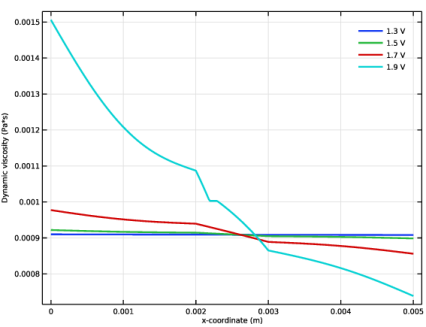
5
In the Label text field, type Fluid Viscosity.
Line Graph 1
1
In the Model Builder window, click Line Graph 1.
2
In the Settings window for Line Graph, locate the y-Axis Data section.
3
In the Expression text field, type fp.mu.
4
In the Fluid Viscosity toolbar, click  Plot.
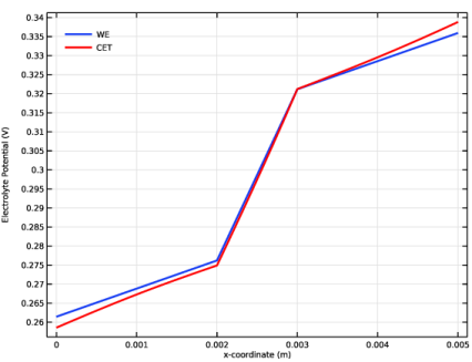
Electrolyte Potential
1
In the Model Builder window, right-click Fluid Viscosity and choose Duplicate.
2
In the Settings window for 1D Plot Group, type Electrolyte Potential in the Label text field.
3
Locate the Plot Settings section.
4
Select the y-axis label checkbox. In the associated text field, type Electrolyte Potential (V).
5
Locate the Legend section. From the Position list, choose Upper left.
Line Graph 1
1
In the Model Builder window, expand the Electrolyte Potential node, then click Line Graph 1.
2
In the Settings window for Line Graph, locate the Data section.
3
From the Dataset list, choose Cut Line 2D 1.
4
Locate the y-Axis Data section. In the Expression text field, type we.phil.
5
Locate the Data section. From the Parameter selection (E_cell) list, choose Last.
6
Locate the Legends section. From the Legends list, choose Manual.
7
Line Graph 2
1
Right-click Results > Electrolyte Potential > Line Graph 1 and choose Duplicate.
2
In the Settings window for Line Graph, locate the Data section.
3
From the Dataset list, choose Cut Line 2D 2.
4
Locate the y-Axis Data section. In the Expression text field, type cet.phil.
5
Locate the Legends section. In the table, enter the following settings:
6
Locate the Coloring and Style section. From the Color list, choose Red.
7
In the Electrolyte Potential toolbar, click  Plot.
Study 1 - WE Only
Finally, disable the Concentrated Electrolyte Transport and Free and Porous Media Flow, Brinkman interfaces and the CET variables in Study 1 to ensure that it can still be solved.
Step 1: Current Distribution Initialization
1
In the Model Builder window, under Study 1 - WE Only click Step 1: Current Distribution Initialization.
2
In the Settings window for Current Distribution Initialization, locate the Physics and Variables Selection section.
3
Select the Modify model configuration for study step checkbox.
4
In the tree, select Component 1 (comp1) > Definitions > Variables - KOH Properties, CET.
5
6
In the tree, select Component 1 (comp1) > Concentrated Electrolyte Transport (cet).
7
Right-click and choose Disable in Model.
8
In the tree, select Component 1 (comp1) > Free and Porous Media Flow, Brinkman (fp).
9
Right-click and choose Disable in Model.
Step 2: Stationary
1
In the Model Builder window, click Step 2: Stationary.
2
In the Settings window for Stationary, locate the Physics and Variables Selection section.
3
Select the Modify model configuration for study step checkbox.
4
In the tree, select Component 1 (comp1) > Definitions > Variables - KOH Properties, CET.
5
6
In the tree, select Component 1 (comp1) > Concentrated Electrolyte Transport (cet).
7
Right-click and choose Disable in Model.
8
In the tree, select Component 1 (comp1) > Free and Porous Media Flow, Brinkman (fp).
9
Right-click and choose Disable in Model.