
|
|
|
|
1.49·107 1/s
|
||

|
3.92·10-7 in
|
||
|
3
|
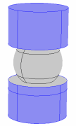
A submodel of the critical joint with a fine mesh is created. The displacements from step 1 are prescribed as Prescribed Displacement on the boundaries where the submodel is cut out of the full model. Similarly, the temperature from step 1 is prescribed as a Temperature in the heat transfer analysis of the submodel. This is done for all time steps of the four simulated cycles.
|
|
4
|
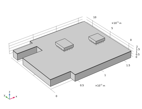
A fatigue analysis is performed on the critical solder joint in the submodel. A life prediction is made based on the energy dissipation in a 50 μm thick layer. Two layers are evaluated. One that is in connection with the copper side and one that is in connection with the microchip side.
|
|
9·103
|
|
1
|
|
2
|
In the Application Libraries window, select Nonlinear Structural Materials Module > Viscoplasticity > viscoplastic_solder_joints in the tree.
|
|
3
|
Click
|
|
1
|
|
2
|
|
1
|
|
2
|
|
1
|
|
2
|
|
3
|
In the Expression text field, type (flc2hs(x-0.1,0.1)*50)*(x<6)-flc2hs(mod(x,6)-4.1,0.1)*40+(flc2hs(mod(x,6)-0.1,0.1)*40+10)*(x>=6).
|
|
1
|
|
2
|
|
3
|
|
4
|
|
1
|
|
2
|
|
1
|
In the Model Builder window, expand the Full Model: Load History node, then click Step 1: Time Dependent.
|
|
2
|
|
3
|
In the Output times text field, type 0 0.005 range(0.025,0.025,0.5) range(0.75,0.25,3.75) 3.975 4+{range(0,0.025,0.5) range(0.75,0.25,2)} 6+{range(0.025,0.025,0.5) range(0.75,0.25,3.75) 3.975 4+{range(0,0.025,0.5) range(0.75,0.25,2)}} 12+{range(0.025,0.025,0.5) range(0.75,0.25,3.75) 3.975 4+{range(0,0.025,0.5) range(0.75,0.25,2)}} 18+{range(0.025,0.025,0.5) range(0.75,0.25,3.75) 3.975 4+{range(0,0.025,0.5) range(0.75,0.25,2)}}.
|
|
1
|
In the Model Builder window, expand the Full Model: Load History > Solver Configurations > Solution 1 (sol1) node.
|
|
2
|
|
1
|
|
2
|
Go to the Add Physics window.
|
|
3
|
|
4
|
Find the Physics interfaces in study subsection. In the table, clear the Solve checkbox for Full Model: Load History.
|
|
5
|
Click the Add to Full Model button in the window toolbar.
|
|
6
|
|
1
|
|
2
|
|
3
|
|
4
|
|
5
|
|
6
|
|
7
|
|
1
|
|
2
|
|
1
|
Go to the Add Study window.
|
|
2
|
Find the Physics interfaces in study subsection. In the table, clear the Solve checkboxes for Solid Mechanics (solid) and Heat Transfer in Solids (ht).
|
|
3
|
Find the Studies subsection. In the Select Study tree, select Preset Studies for Selected Physics Interfaces > Fatigue.
|
|
4
|
Click the Add Study button in the window toolbar.
|
|
5
|
|
1
|
In the Model Builder window, expand the Solder, 60Sn-40Pb (mat4) node, then click Full Model: Fatigue Evaluation > Step 1: Fatigue.
|
|
2
|
|
3
|
Find the Values of variables not solved for subsection. From the Settings list, choose User controlled.
|
|
4
|
|
5
|
|
6
|
|
8
|
|
1
|
|
2
|
|
3
|
Click
|
|
4
|
Browse to the model’s Application Libraries folder and double-click the file viscoplastic_solder_joints.mphbin.
|
|
5
|
Click
|
|
1
|
|
2
|
|
3
|
|
4
|
|
5
|
|
6
|
|
7
|
|
1
|
|
2
|
|
1
|
|
2
|
Click in the Graphics window and then press Ctrl+A to select both objects.
|
|
1
|
|
2
|
|
3
|
|
4
|
|
1
|
|
2
|
|
3
|
|
1
|
|
2
|
|
3
|
|
4
|
|
5
|
|
6
|
|
7
|
Select the object int1 only.
|
|
1
|
|
2
|
Select the object par1 only.
|
|
3
|
|
4
|
|
5
|
Click
|
|
6
|
|
1
|
|
2
|
Go to the Add Physics window.
|
|
3
|
|
4
|
Find the Physics interfaces in study subsection. In the table, clear the Solve checkboxes for Full Model: Load History and Full Model: Fatigue Evaluation.
|
|
5
|
Click the Add to Submodel button in the window toolbar.
|
|
6
|
|
1
|
|
2
|
From the list, choose Quasistatic.
|
|
1
|
|
2
|
In the Show More Options dialog, in the tree, select the checkbox for the node Physics > Advanced Physics Options.
|
|
3
|
Click OK.
|
|
4
|
In the Model Builder window, under Submodel (comp2) > Solid Mechanics 2 (solid2) click Linear Elastic Material 1.
|
|
5
|
|
6
|
|
1
|
|
2
|
|
3
|
Click
|
|
1
|
|
3
|
|
4
|
|
5
|
|
6
|
|
7
|
|
8
|
|
9
|
|
10
|
Click to expand the Constraint Settings section. From the Apply reaction terms on list, choose Current physics (internally symmetric).
|
|
1
|
|
3
|
|
4
|
|
1
|
|
3
|
|
4
|
|
5
|
|
6
|
|
1
|
|
3
|
|
4
|
|
1
|
In the Model Builder window, under Submodel (comp2) right-click Materials and choose More Materials > Material Link.
|
|
1
|
|
3
|
|
4
|
|
1
|
|
3
|
|
4
|
|
1
|
|
3
|
|
4
|
|
1
|
|
2
|
|
3
|
From the list, choose User-controlled mesh.
|
|
1
|
|
2
|
|
3
|
|
5
|
|
6
|
|
7
|
Click
|
|
1
|
|
2
|
Go to the Add Study window.
|
|
3
|
Find the Physics interfaces in study subsection. In the table, clear the Solve checkboxes for Solid Mechanics (solid), Heat Transfer in Solids (ht), and Fatigue (ftg).
|
|
4
|
|
5
|
Click the Add Study button in the window toolbar.
|
|
6
|
|
1
|
|
2
|
|
3
|
|
4
|
In the Output times text field, type 0 range(1,1,17) 18+{range(0,0.025,0.5) range(0.75,0.25,3.75) 3.95 4+{range(0.025,0.025,0.5) range(0.75,0.25,2)}}.
|
|
5
|
Click to expand the Values of Dependent Variables section. Find the Values of variables not solved for subsection. From the Settings list, choose User controlled.
|
|
6
|
|
7
|
|
8
|
|
1
|
|
2
|
|
3
|
|
4
|
|
5
|
|
6
|
In the Model Builder window, expand the Submodel: Load History > Solver Configurations > Solution 4 (sol4) > Time-Dependent Solver 1 node, then click Segregated 1.
|
|
7
|
|
8
|
|
9
|
In the Model Builder window, expand the Submodel: Load History > Solver Configurations > Solution 4 (sol4) > Time-Dependent Solver 1 > Segregated 1 node, then click Temperature.
|
|
10
|
|
11
|
|
12
|
|
13
|
In the Model Builder window, under Submodel: Load History > Solver Configurations > Solution 4 (sol4) > Time-Dependent Solver 1 > Segregated 1 click Solid Mechanics 2.
|
|
14
|
|
15
|
|
16
|
|
17
|
|
18
|
|
1
|
|
2
|
Go to the Add Physics window.
|
|
3
|
|
4
|
Find the Physics interfaces in study subsection. In the table, clear the Solve checkboxes for Full Model: Load History, Full Model: Fatigue Evaluation, and Submodel: Load History.
|
|
5
|
Click the Add to Submodel button in the window toolbar.
|
|
6
|
|
1
|
|
3
|
|
4
|
|
5
|
|
6
|
|
7
|
Locate the Evaluation Settings section. From the Volume average method list, choose Entire selection.
|
|
8
|
|
1
|
|
2
|
Go to the Add Physics window.
|
|
3
|
|
4
|
Find the Physics interfaces in study subsection. In the table, clear the Solve checkboxes for Full Model: Load History, Full Model: Fatigue Evaluation, and Submodel: Load History.
|
|
5
|
Click the Add to Submodel button in the window toolbar.
|
|
6
|
|
2
|
|
3
|
|
4
|
|
5
|
|
6
|
|
1
|
|
2
|
Go to the Add Study window.
|
|
3
|
Find the Physics interfaces in study subsection. In the table, clear the Solve checkboxes for Solid Mechanics (solid), Heat Transfer in Solids (ht), Fatigue (ftg), Solid Mechanics 2 (solid2), and Heat Transfer in Solids 2 (ht2).
|
|
4
|
Find the Studies subsection. In the Select Study tree, select Preset Studies for Selected Physics Interfaces > Fatigue.
|
|
5
|
Click the Add Study button in the window toolbar.
|
|
6
|
|
1
|
|
2
|
|
3
|
Find the Values of variables not solved for subsection. From the Settings list, choose User controlled.
|
|
4
|
|
5
|
|
6
|
|
8
|
|
1
|
|
2
|
|
3
|
|
4
|
|
1
|
|
2
|
|
3
|
Select the Show legends checkbox.
|
|
4
|
|
1
|
|
2
|
|
3
|
|
4
|
|
5
|
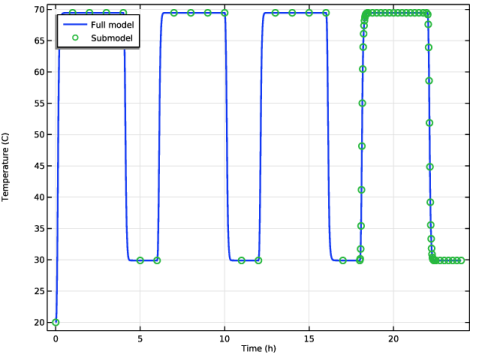
Locate the Data section. From the Dataset list, choose Submodel: Load History/Solution 4 (5) (sol4).
|
|
6
|
|
8
|
Click to expand the Coloring and Style section. Find the Line markers subsection. From the Marker list, choose Circle.
|
|
9
|
Locate the Legends section. In the table, enter the following settings:
|
|
1
|
|
2
|
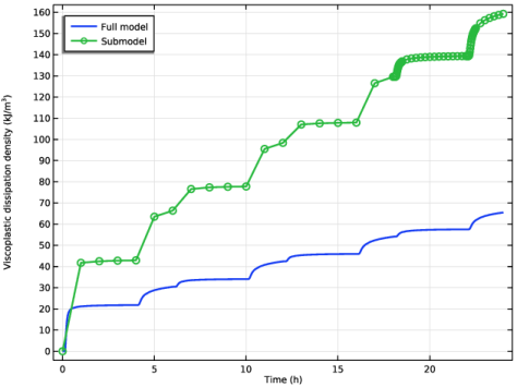
In the Settings window for 1D Plot Group, type Shear Viscoplasticity History in the Label text field.
|
|
3
|
Locate the Plot Settings section.
|
|
4
|
|
5
|
|
1
|
In the Model Builder window, expand the Shear Viscoplasticity History node, then click Point Graph 1.
|
|
2
|
In the Settings window for Point Graph, click Replace Expression in the upper-right corner of the y-Axis Data section. From the menu, choose Full Model (comp1) > Solid Mechanics > Strain > Viscoplastic strain tensor, local coordinate system > solid.evplGp13 - Viscoplastic strain tensor, local coordinate system, 13-component.
|
|
1
|
|
2
|
In the Settings window for Point Graph, click Replace Expression in the upper-right corner of the y-Axis Data section. From the menu, choose Submodel (comp2) > Solid Mechanics 2 > Strain > Viscoplastic strain tensor, local coordinate system > solid2.evplGp13 - Viscoplastic strain tensor, local coordinate system, 13-component.
|
|
3
|
|
1
|
|
2
|
|
3
|
|
4
|
Locate the Plot Settings section.
|
|
5
|
|
6
|
|
1
|
|
2
|
|
3
|
Select the Show legends checkbox.
|
|
4
|
|
1
|
|
2
|
|
3
|
|
4
|
|
5
|
Locate the Data section. From the Dataset list, choose Submodel: Load History/Solution 4 (5) (sol4).
|
|
6
|
|
8
|
Locate the Coloring and Style section. Find the Line style subsection. From the Line list, choose None.
|
|
9
|
|
10
|
Locate the Legends section. In the table, enter the following settings:
|
|
1
|
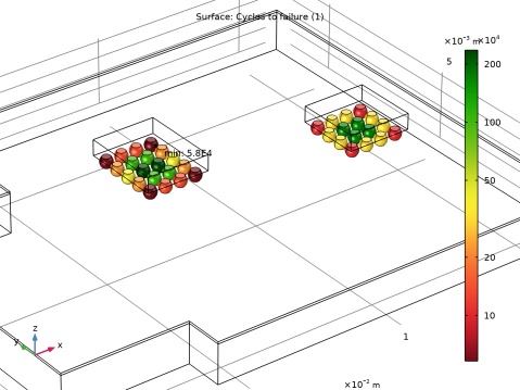
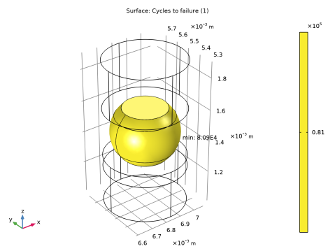
In the Model Builder window, expand the Results > Cycles to Failure (ftg) > Surface 1 node, then click Marker 1.
|
|
2
|
|
3
|
|
1
|
|
2
|
|
1
|
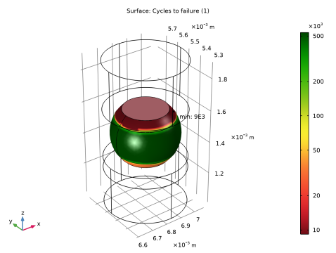
In the Model Builder window, expand the Results > Cycles to Failure (ftg3) > Surface 1 node, then click Marker 1.
|
|
2
|
|
3
|
|
1
|
|
2
|
|
3
|
|
4
|
|
5
|
Click Replace Expression in the upper-right corner of the Expressions section. From the menu, choose Full Model (comp1) > Fatigue > ftg.ctf - Cycles to failure - 1.
|
|
1
|
|
2
|
|
3
|
|
5
|
Locate the Expressions section. In the table, enter the following settings:
|
|
6
|