|
|
|


|
1
|
|
2
|
|
3
|
Click Add.
|
|
4
|
Click
|
|
5
|
|
6
|
Click
|
|
1
|
|
2
|
|
1
|
|
2
|
|
3
|
|
1
|
|
2
|
|
3
|
|
4
|
|
1
|
|
2
|
|
3
|
|
4
|
|
5
|
|
1
|
|
2
|
|
3
|
|
4
|
|
5
|
|
6
|
|
1
|
|
2
|
|
3
|
|
4
|
|
5
|
|
1
|
|
2
|
|
3
|
|
4
|
|
5
|
|
6
|
|
7
|
|
8
|
|
1
|
|
2
|
|
3
|
|
4
|
|
1
|
In the Model Builder window, under Component 1 (comp1) > Solid Mechanics (solid) click Linear Elastic Material 1.
|
|
2
|
|
3
|
|
4
|
|
5
|
|
1
|
|
2
|
|
3
|
Click
|
|
5
|
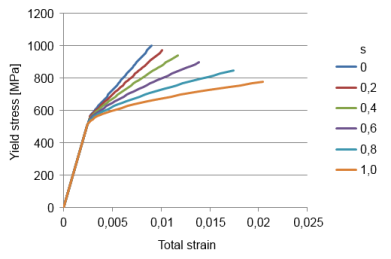
Locate the Plasticity Model section. From the σys0 list, choose User defined. In the associated text field, type 570[MPa].
|
|
6
|
Find the Isotropic hardening model subsection. From the ETiso list, choose User defined. In the associated text field, type 69[GPa].
|
|
1
|
In the Model Builder window, under Component 1 (comp1) > Solid Mechanics (solid) > Linear Elastic Material 1 click Plasticity 1.
|
|
2
|
|
1
|
In the Model Builder window, under Component 1 (comp1) > Solid Mechanics (solid) > Linear Elastic Material 1 click Plasticity 2.
|
|
2
|
|
3
|
|
5
|
Locate the Plasticity Model section. From the σys0 list, choose User defined. In the associated text field, type 515[MPa].
|
|
6
|
|
7
|
|
8
|
|
1
|
|
2
|
|
3
|
Locate the Definition section. In the table, enter the following settings:
|
|
4
|
|
1
|
In the Model Builder window, under Component 1 (comp1) right-click Definitions and choose Variables.
|
|
2
|
|
1
|
|
2
|
|
3
|
|
5
|
Locate the Plasticity Model section. From the σys0 list, choose User defined. In the associated text field, type s0T.
|
|
6
|
|
7
|
|
8
|
|
1
|
|
2
|
|
3
|
Locate the Definition section. In the table, enter the following settings:
|
|
4
|
|
1
|
|
2
|
|
3
|
|
1
|
|
1
|
|
2
|
|
3
|
|
1
|
|
2
|
|
1
|
|
3
|
|
4
|
|
5
|
|
1
|
|
2
|
|
3
|
|
1
|
|
3
|
|
4
|
|
1
|
|
3
|
|
4
|
|
1
|
|
3
|
|
4
|
|
1
|
|
2
|
|
1
|
|
2
|
|
3
|
Select the Auxiliary sweep checkbox.
|
|
4
|
Click
|
|
6
|
|
1
|
|
2
|
|
3
|
Click
|
|
4
|
|
5
|
Click OK.
|
|
6
|
|
8
|
Click
|
|
1
|
|
2
|
|
3
|
|
1
|
|
2
|
|
3
|
|
1
|
|
2
|
|
1
|
|
2
|
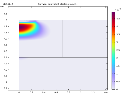
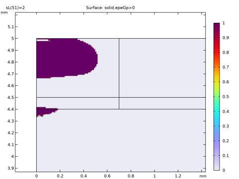
In the Settings window for Surface, click Replace Expression in the upper-right corner of the Expression section. From the menu, choose Component 1 (comp1) > Solid Mechanics > Strain > solid.epeGp - Equivalent plastic strain - 1.
|
|
3
|
|
1
|
|
2
|
|
1
|
|
2
|
|
1
|
|
2
|
|
3
|
|
1
|
|
2
|
|
1
|
|
2
|
|
4
|
|
1
|
|
2
|
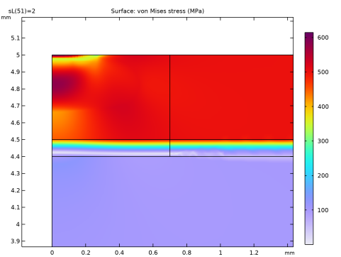
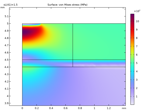
In the Settings window for 2D Plot Group, type Equivalent stress at peak load in the Label text field.
|
|
3
|
|
1
|
|
2
|
|
3
|
|
1
|
|
2
|
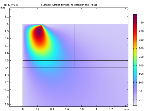
In the Settings window for Surface, click Replace Expression in the upper-right corner of the Expression section. From the menu, choose Component 1 (comp1) > Solid Mechanics > Stress > Stress tensor (spatial frame) - N/m² > solid.sGprz - Stress tensor, rz-component.
|
|
3
|
|
1
|
|
2
|
Go to the Add Physics window.
|
|
3
|
|
4
|
Find the Physics interfaces in study subsection. In the table, clear the Solve checkbox for Study 1.
|
|
5
|
Click the Add to Component 1 button in the window toolbar.
|
|
1
|
|
2
|
|
3
|
|
4
|
|
5
|
|
6
|
|
1
|
In the Model Builder window, under Component 1 (comp1) right-click Materials and choose Blank Material.
|
|
2
|
|
3
|
Click
|
|
5
|
Locate the Material Contents section. In the table, enter the following settings:
|
|
1
|
|
3
|
|
1
|
|
2
|
Go to the Add Study window.
|
|
3
|
Find the Physics interfaces in study subsection. In the table, clear the Solve checkbox for Solid Mechanics (solid).
|
|
4
|
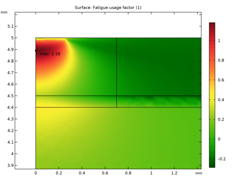
Find the Studies subsection. In the Select Study tree, select Preset Studies for Selected Physics Interfaces > Fatigue.
|
|
5
|
Click the Add Study button in the window toolbar.
|
|
6
|
|
1
|
|
2
|
Find the Values of variables not solved for subsection. From the Settings list, choose User controlled.
|
|
3
|
|
4
|
|
5
|
|
6
|
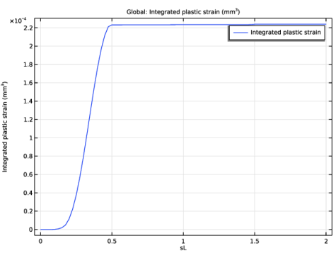
In the Parameter value (sL) list, choose 0.6, 0.65, 0.7, 0.75, 0.8, 0.85, 0.9, 0.95, 1, 1.05, 1.1, 1.15, 1.2, 1.25, 1.3, 1.35, 1.4, 1.45, 1.5, 1.55, and 1.6.
|
|
7
|