

PDF

Fatigue Analysis of a Wheel Rim
Introduction
During the development of safety-critical components like a car wheel rim, making sure fatigue cracks do not occur is one of the most important tasks. When a final prototype is available this is ensured by testing, but prototype production and testing are time-consuming and expensive activities. Good predictions from simulations can keep the number of prototypes to a minimum.
In this example, you perform a fatigue evaluation on a model of a wheel rim, subjected to the load history from a simulated test.
Model Definition
For a definition of geometry, loads, and boundary conditions, see the documentation for the model Submodel in a Wheel Rim in the Structural Mechanics Module Application Library.
The fatigue limit (in terms if the stress amplitude) is known for two cases with pure axial loading. For pure tension it is 95 MPa, and for fully reversed loading it is 125 MPa. In this model, you use the Findley criterion, so the Findley parameters have to be derived from these data.
In pure tension, the Findley criterion can be written as
This means that you have to solve the simultaneous equations
to get the Findley parameters f and k. The result is f = 84 MPa and k = 0.30.
Results and Discussion
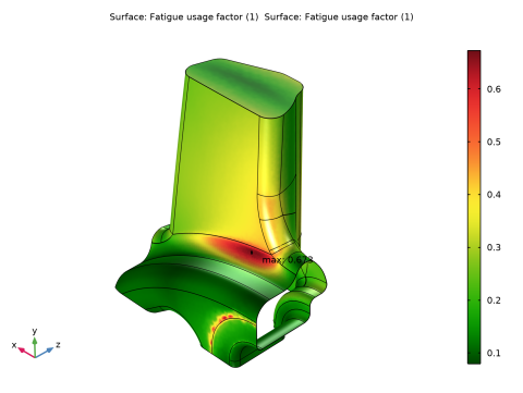
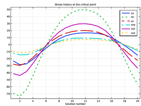
The fatigue usage factor distribution is shown in Figure 1. The maximum value is about 0.666, which should indicate that the design is good when taking into account that the required safety factor has been included in the load. In Figure 2, the stress histories at the critical point are displayed. The loading is slightly nonproportional, and has a compressive mean stress, which is captured by the Findley criterion.
Figure 1: Fatigue usage factor using the Findley criterion.
Figure 2: Stress histories at the critical point.
Notes About the COMSOL Implementation
In this example, you perform the fatigue analysis as an additional study step in a model that already contains the results from a stress analysis. Because the critical points for fatigue crack initiation is on the free surface of the body, it is sufficient to do the fatigue evaluation on the boundary and not in the domain. This approach reduces the CPU and memory requirements significantly.
Application Library path: Fatigue_Module/Stress_Based/rim_fatigue
Modeling Instructions
Root
In this example you will start from an existing model which is an example in the Structural Mechanics Module.
Application Libraries
1
From the File menu, choose Application Libraries.
2
In the Application Libraries window, select Structural Mechanics Module > Tutorials > rim_submodel in the tree.
3
Add a selection to help with the physics setup.
Component 2 (comp2)
In the Model Builder window, expand the Component 2 (comp2) node.
Geometry 2
In the Model Builder window, expand the Component 2 (comp2) > Geometry 2 node.
Fatigue Evaluation
1
In the Model Builder window, expand the Component 2 (comp2) > Geometry 2 > Selections node.
2
Right-click Selections and choose Selections > Complement Selection.
3
In the Settings window for Complement Selection, type Fatigue Evaluation in the Label text field.
4
Locate the Geometric Entity Level section. From the Level list, choose Boundary.
5
Locate the Input Entities section. Click  Add.
6
In the Add dialog, in the Selections to invert list, choose Prescribed Displacement and Fixed to Hub.
7
Results
Stress in Submodel
If the model was stored without solutions, you will now have to run Study 1 and Study 2 before continuing.
Add Physics
1
In the Home toolbar, click  Add Physics to open the Add Physics window.
2
Go to the Add Physics window.
3
In the tree, select Structural Mechanics > Fatigue (ftg).
4
Find the Physics interfaces in study subsection. In the table, clear the Solve checkboxes for Study 1 and Study 2.
5
Click the Add to Component 2 button in the window toolbar.
6
In the Home toolbar, click  Add Physics to close the Add Physics window.
Fatigue (ftg)
Stress-Based 1
1
In the Physics toolbar, click  Boundaries and choose Stress-Based.
2
In the Settings window for Stress-Based, locate the Boundary Selection section.
3
From the Selection list, choose Fatigue Evaluation.
4
Locate the Solution Field section. From the Physics interface list, choose Solid Mechanics 2 (solid2).
Materials
Material 5 (mat5)
1
In the Model Builder window, expand the Component 2 (comp2) > Materials node.
2
Right-click Component 2 (comp2) > Materials and choose Blank Material.
3
In the Settings window for Material, locate the Geometric Entity Selection section.
4
From the Geometric entity level list, choose Boundary.
5
From the Selection list, choose Fatigue Evaluation.
6
Locate the Material Contents section. In the table, enter the following settings:
Add Study
1
In the Home toolbar, click  Add Study to open the Add Study window.
2
Go to the Add Study window.
3
Find the Physics interfaces in study subsection. In the table, clear the Solve checkboxes for Solid Mechanics (solid) and Solid Mechanics 2 (solid2).
4
Find the Studies subsection. In the Select Study tree, select Preset Studies for Selected Physics Interfaces > Fatigue.
5
Click the Add Study button in the window toolbar.
6
In the Home toolbar, click  Add Study to close the Add Study window.
Study 3
Step 1: Fatigue
1
In the Settings window for Fatigue, locate the Values of Dependent Variables section.
2
Find the Values of variables not solved for subsection. From the Settings list, choose User controlled.
3
From the Method list, choose Solution.
4
From the Study list, choose Study 2, Stationary.
5
In the Study toolbar, click  Compute.
Results
Fatigue Usage Factor (ftg)
1
In the Fatigue Usage Factor (ftg) toolbar, click  Plot.
2
In the Model Builder window, click Fatigue Usage Factor (ftg).
3
In the Settings window for 3D Plot Group, locate the Plot Settings section.
4
From the View list, choose View 4.
In order to get the location of the point with maximum fatigue usage, zoom in on the maximum marker and click on it in the graphics window. You will then see the value and the coordinates in the Table window. The location will be approximately (0.017, 0.092, 0.088). Use these coordinates to create a Cut Point 3D dataset for detailed evaluation of the stress history in the critical point.
Cut Point 3D 1
1
In the Results toolbar, click  Cut Point 3D.
2
In the Settings window for Cut Point 3D, locate the Data section.
3
From the Dataset list, choose Study 2/Solution 2 (3) (sol2).
4
Locate the Point Data section. In the X text field, type 0.017.
5
In the Y text field, type 0.092.
6
In the Z text field, type 0.088.
7
From the Snapping list, choose Snap to closest boundary.
1D Plot Group 5
In the Results toolbar, click  1D Plot Group.
Point Graph 1
1
Right-click 1D Plot Group 5 and choose Point Graph.
2
In the Settings window for Point Graph, locate the Data section.
3
From the Dataset list, choose Cut Point 3D 1.
4
Click Replace Expression in the upper-right corner of the y-Axis Data section. From the menu, choose Component 2 (comp2) > Solid Mechanics 2 > Stress > Stress tensor (spatial frame) - N/m² > solid2.sGpxx - Stress tensor, xx-component.
5
Locate the y-Axis Data section. From the Unit list, choose MPa.
6
Click to expand the Coloring and Style section. Find the Line style subsection. From the Line list, choose Cycle.
7
Locate the x-Axis Data section. From the Axis source data list, choose All solutions.
8
Locate the Coloring and Style section. From the Width list, choose 3.
9
Click to expand the Legends section. Select the Show legends checkbox.
10
From the Legends list, choose Manual.
11
Point Graph 2
1
Right-click Point Graph 1 and choose Duplicate.
2
In the Settings window for Point Graph, locate the y-Axis Data section.
3
In the Expression text field, type solid2.sy.
4
Locate the Legends section. In the table, enter the following settings:
Point Graph 3
1
Right-click Point Graph 2 and choose Duplicate.
2
In the Settings window for Point Graph, locate the y-Axis Data section.
3
In the Expression text field, type solid2.sz.
4
Locate the Legends section. In the table, enter the following settings:
Point Graph 4
1
Right-click Point Graph 3 and choose Duplicate.
2
In the Settings window for Point Graph, locate the y-Axis Data section.
3
In the Expression text field, type solid2.sxy.
4
Locate the Legends section. In the table, enter the following settings:
Point Graph 5
1
Right-click Point Graph 4 and choose Duplicate.
2
In the Settings window for Point Graph, locate the y-Axis Data section.
3
In the Expression text field, type solid2.syz.
4
Locate the Legends section. In the table, enter the following settings:
Point Graph 6
1
Right-click Point Graph 5 and choose Duplicate.
2
In the Settings window for Point Graph, locate the y-Axis Data section.
3
In the Expression text field, type solid2.sxz.
4
Locate the Legends section. In the table, enter the following settings:
Stress History
1
In the Model Builder window, under Results click 1D Plot Group 5.
2
In the Settings window for 1D Plot Group, type Stress History in the Label text field.
3
Click to expand the Title section. From the Title type list, choose Manual.
4
In the Title text area, type Stress history at the critical point.
5
In the Stress History toolbar, click  Plot.