|
|
|
|
•
|
|
•
|
|
•
|
|
1
|
|
2
|
|
3
|
Click Add.
|
|
4
|
Click
|
|
5
|
|
6
|
Click
|
|
1
|
|
2
|
|
3
|
|
1
|
|
2
|
|
3
|
Click
|
|
4
|
Browse to the model’s Application Libraries folder and double-click the file linear_guide_geometry.mphbin.
|
|
5
|
Click
|
|
1
|
|
2
|
|
3
|
Click the
|
|
1
|
|
2
|
|
3
|
|
1
|
|
2
|
|
3
|
|
5
|
|
1
|
|
2
|
|
3
|
Click
|
|
4
|
Browse to the model’s Application Libraries folder and double-click the file linear_guide_parameters.txt.
|
|
1
|
In the Model Builder window, under Component 1 (comp1) right-click Definitions and choose Variables.
|
|
2
|
|
3
|
Click
|
|
4
|
Browse to the model’s Application Libraries folder and double-click the file linear_guide_variables.txt.
|
|
1
|
|
2
|
|
3
|
|
4
|
|
1
|
In the Model Builder window, under Component 1 (comp1) right-click Materials and choose Blank Material.
|
|
2
|
|
1
|
|
2
|
|
3
|
|
4
|
|
5
|
|
1
|
|
1
|
|
1
|
|
2
|
|
3
|
|
1
|
|
2
|
|
3
|
|
4
|
Click to expand the Element Size Parameters section. Locate the Element Size section. Click the Custom button.
|
|
5
|
Locate the Element Size Parameters section.
|
|
6
|
|
1
|
|
2
|
|
3
|
|
4
|
|
1
|
|
2
|
|
3
|
|
1
|
|
2
|
|
3
|
|
4
|
|
5
|
|
6
|
|
7
|
Select the Reverse direction checkbox.
|
|
1
|
|
2
|
|
3
|
Click the Custom button.
|
|
4
|
Locate the Element Size Parameters section.
|
|
5
|
|
6
|
Click
|
|
1
|
|
2
|
|
3
|
Select the Auxiliary sweep checkbox.
|
|
4
|
Click
|
|
1
|
|
2
|
|
3
|
In the Model Builder window, expand the Study 1 > Solver Configurations > Solution 1 (sol1) > Stationary Solver 1 node.
|
|
4
|
Right-click Study 1 > Solver Configurations > Solution 1 (sol1) > Stationary Solver 1 > Suggested Iterative Solver (solid) and choose Enable.
|
|
5
|
|
1
|
|
2
|
|
3
|
Click
|
|
4
|
|
5
|
Click OK.
|
|
6
|
|
8
|
Click
|
|
1
|
|
2
|
|
3
|
|
4
|
|
1
|
|
2
|
|
3
|
|
4
|
|
5
|
Locate the Plot Settings section. From the View list, choose New view to create a dedicated view for this plot.
|
|
6
|
|
1
|
|
2
|
|
3
|
|
5
|
|
1
|
|
2
|
|
3
|
|
4
|
|
1
|
|
2
|
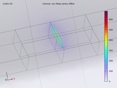
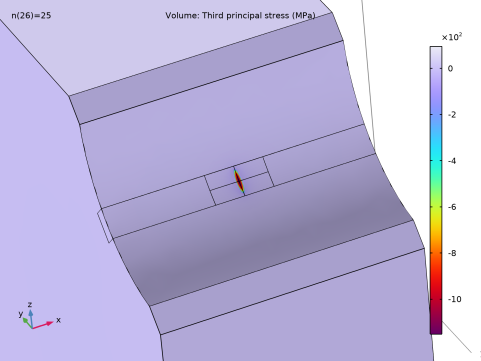
In the Settings window for Volume, click Replace Expression in the upper-right corner of the Expression section. From the menu, choose Component 1 (comp1) > Solid Mechanics > Stress > Principal stresses > solid.sp3Gp - Third principal stress - N/m².
|
|
3
|
|
1
|
|
2
|
In the Settings window for Cut Plane, type Study1/Cut Plane: Through Thickness in the Label text field.
|
|
1
|
|
2
|
In the Settings window for 2D Plot Group, type Subsurface: Equivalent Stress in the Label text field.
|
|
3
|
|
4
|
|
5
|
|
1
|
|
2
|
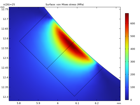
In the Settings window for Surface, click Replace Expression in the upper-right corner of the Expression section. From the menu, choose Component 1 (comp1) > Solid Mechanics > Stress > solid.misesGp - von Mises stress - N/m².
|
|
1
|
|
2
|
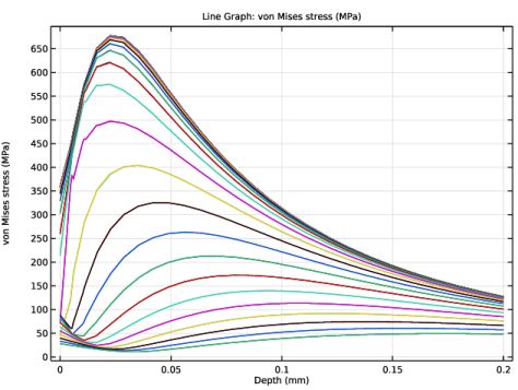
In the Settings window for 1D Plot Group, type Through Thickness: Equivalent Stress in the Label text field.
|
|
1
|
|
2
|
|
3
|
|
4
|
Click Replace Expression in the upper-right corner of the y-Axis Data section. From the menu, choose Component 1 (comp1) > Solid Mechanics > Stress > solid.misesGp - von Mises stress - N/m².
|
|
5
|
|
1
|
|
2
|
|
3
|
|
1
|
|
2
|
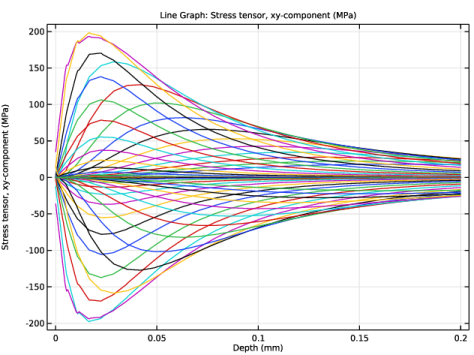
In the Settings window for 1D Plot Group, type Through Thickness: Shear Stress in the Label text field.
|
|
1
|
In the Model Builder window, expand the Through Thickness: Shear Stress node, then click Line Graph 1.
|
|
2
|
In the Settings window for Line Graph, click Replace Expression in the upper-right corner of the y-Axis Data section. From the menu, choose Component 1 (comp1) > Solid Mechanics > Stress > Stress tensor (spatial frame) - N/m² > solid.sGpxy - Stress tensor, xy-component.
|
|
1
|
|
2
|
|
3
|
|
4
|
|
5
|
|
1
|
|
2
|
|
3
|
|
4
|
|
1
|
|
2
|
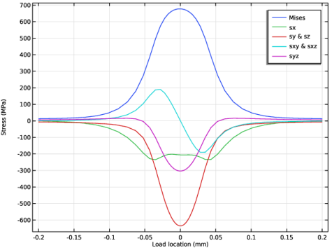
In the Settings window for 1D Plot Group, type Point of Max Mises: Stress Components in the Label text field.
|
|
3
|
|
1
|
|
2
|
In the Settings window for Point Graph, click Replace Expression in the upper-right corner of the y-Axis Data section. From the menu, choose Component 1 (comp1) > Solid Mechanics > Stress > solid.misesGp - von Mises stress - N/m².
|
|
3
|
|
4
|
|
5
|
|
6
|
|
1
|
|
2
|
In the Settings window for Point Graph, click Replace Expression in the upper-right corner of the y-Axis Data section. From the menu, choose Component 1 (comp1) > Solid Mechanics > Stress > Stress tensor (spatial frame) - N/m² > solid.sGpxx - Stress tensor, xx-component.
|
|
3
|
Locate the Legends section. In the table, enter the following settings:
|
|
1
|
|
2
|
In the Settings window for Point Graph, click Replace Expression in the upper-right corner of the y-Axis Data section. From the menu, choose Component 1 (comp1) > Solid Mechanics > Stress > Stress tensor (spatial frame) - N/m² > solid.sGpyy - Stress tensor, yy-component.
|
|
3
|
Locate the Legends section. In the table, enter the following settings:
|
|
1
|
|
2
|
In the Settings window for Point Graph, click Replace Expression in the upper-right corner of the y-Axis Data section. From the menu, choose Component 1 (comp1) > Solid Mechanics > Stress > Stress tensor (spatial frame) - N/m² > solid.sGpxy - Stress tensor, xy-component.
|
|
3
|
Locate the Legends section. In the table, enter the following settings:
|
|
1
|
|
2
|
In the Settings window for Point Graph, click Replace Expression in the upper-right corner of the y-Axis Data section. From the menu, choose Component 1 (comp1) > Solid Mechanics > Stress > Stress tensor (spatial frame) - N/m² > solid.sGpyz - Stress tensor, yz-component.
|
|
3
|
Locate the Legends section. In the table, enter the following settings:
|
|
4
|
|
1
|
|
2
|
|
3
|
|
4
|
Locate the Plot Settings section.
|
|
5
|
|
6
|
|
7
|
|
1
|
|
2
|
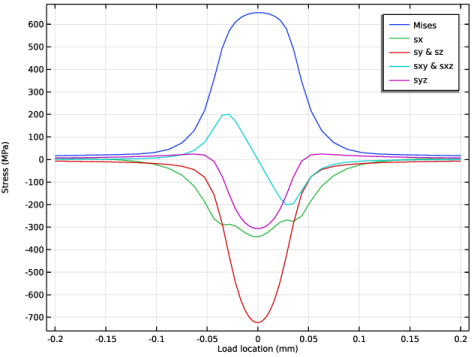
In the Settings window for 1D Plot Group, type Point of Max Shear: Stress Components in the Label text field.
|
|
3
|
|
4
|
|
1
|
|
2
|
Go to the Add Physics window.
|
|
3
|
|
4
|
Find the Physics interfaces in study subsection. In the table, clear the Solve checkbox for Study 1.
|
|
5
|
Click the Add to Component 1 button in the window toolbar.
|
|
6
|
|
1
|
|
2
|
|
3
|
|
4
|
|
5
|
|
1
|
|
2
|
|
1
|
|
2
|
Go to the Add Study window.
|
|
3
|
Find the Physics interfaces in study subsection. In the table, clear the Solve checkbox for Solid Mechanics (solid).
|
|
4
|
Find the Studies subsection. In the Select Study tree, select Preset Studies for Selected Physics Interfaces > Fatigue.
|
|
5
|
Click the Add Study button in the window toolbar.
|
|
6
|
|
1
|
|
2
|
Find the Values of variables not solved for subsection. From the Settings list, choose User controlled.
|
|
3
|
|
4
|
|
5
|
|
1
|
|
2
|
|
3
|
|
4
|
|
1
|
|
2
|
|
3
|
|
1
|
|
2
|
|
3
|
|
4
|
|
1
|
|
2
|
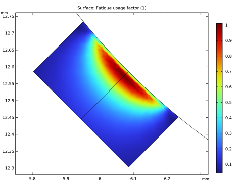
In the Settings window for 2D Plot Group, type Subsurface: Fatigue Usage Factor in the Label text field.
|
|
3
|
|
4
|
|
1
|
|
2
|
In the Settings window for Surface, click Replace Expression in the upper-right corner of the Expression section. From the menu, choose Component 1 (comp1) > Fatigue > ftg.fus - Fatigue usage factor - 1.
|
|
3
|