PDF

Positive Streamer Propagation in a Weak Electric Field
Introduction
Understanding the dynamics of positive streamer propagation in weak electric fields is pivotal in various scientific and technological realms, ranging from atmospheric physics to plasma-based technologies. Positive streamers, characterized by their filamentary structure and rapid advancement, play a crucial role in phenomena such as lightning initiation, corona discharges, and electrical breakdown in gases. In this numerical modeling study, we delve into the intricate mechanisms governing the evolution of positive streamers in low electric fields.
One indispensable process driving positive streamer propagation is photoionization, which serves as a fundamental precursor. Photoionization facilitates the generation of seed electrons, thereby enabling subsequent impact ionization at the streamer head. This interplay between photoionization and impact ionization orchestrates the initiation and sustenance of positive streamers in weak electric fields, shaping their intricate morphological characteristics and propagation dynamics.
This case study investigates a positive streamer between point-plate electrodes. Initially, a cluster of electrons and ions is positioned between two electrodes spaced 1 cm apart, subject to a 13 kV voltage. The simulated electric field and electron density is in good agreement with that published in Ref. 1.
Model Definition
The model is two-dimensional and describes the transient behavior of an initial electron seed in the presence of a weak electric field. The Electric Discharge interface is used to simulate the streamer propagation. The built-in charge transport model is used:
where
e, p, n denote electrons, positive ions, and negative ions
ni is the number density of the charge carrier (SI unit: 1/m3)
E is the electric field (SI unit: V/m)
zi denotes the carrier charge (SI unit: 1)
μi denotes the carrier mobility (SI unit: m2/(V·s))
wi is the drift velocity in the electric field (SI unit: m/s)
Di is the diffusion coefficient (SI unit: m2/s)
Ri is the reaction rate (SI unit: 1/(m3·s))
α is the ionization coefficient (SI unit: 1/m)
η is the attachment coefficient (SI unit: 1/m)
βep is the electron–ion recombination coefficient (SI unit: m3/s)
βpn is the ion–ion recombination coefficient (SI unit: m3/s)
The above transport equations are fully coupled with Poisson’s equation through the electric field and the space charge:
where e is the elementary charge.
For atmospheric pressure positive discharges, photoionization is critical. This model uses the radiative transfer model for computing photoionization. See the section on Photoionization in the Electric Discharge Module User’s Guide for further details.
where
Sphjdenotes jth photoionization rate component (SI unit: 1/(m3·s))
pp is the partial pressure (default value: 150 Torr)
p is the gas pressure (default value: 760 Torr)
pq is the quenching pressure (default value: 30 Torr)
ξνui is the photoionization parameter (default value: 0.06)
Aj and λj are fitting parameter
Iph is the effective ionization intensity (SI unit: 1/(m3·s))
Sion is the impact ionization rate (SI unit: 1/(m3·s))
Results and Discussion
The axial electric field and electron number density for several instants during the streamer propagation are shown in Figure 1 and Figure 2, respectively. Figure 3 shows the photoionization rate at t = 23 ns.
The mesh dependency observed in the numerical modeling of positive streamer propagation underscores the intricate balance between mesh resolution and computational accuracy. As noted, the results of the simulations are sensitive to changes in mesh refinement, highlighting the need for careful consideration in mesh selection to adequately capture the nonlinear dynamics inherent in streamer propagation.
A key aspect contributing to mesh dependency is the challenge of resolving the highly nonlinear nature of streamer dynamics. The current mesh employed in the simulations may not possess sufficient resolution to accurately represent the intricate streamer evolution details. Consequently, as the mesh is refined, the results may exhibit variations due to better resolution of the underlying physics.
Interestingly, while mesh refinement introduces instability into the numerical scheme, this instability is instrumental in reproducing the filamentary structure characteristics of streamers. The interplay between mesh-induced instability and the inherent nonlinear dynamics of streamers gives rise to the formation of filamentary structures, crucial for accurately modeling streamer propagation.
Moreover, it is worth noting that separate studies have indicated that, under certain conditions, the model converges to a state where only a diffusive glow corona is formed. This convergence highlights the importance of considering the broader context of streamer dynamics and the limitations of numerical models in capturing all aspects of the phenomenon.
Referring to prior research, it is evident that mesh dependency can arise from various sources. For instance, in Ref. 1, adaptive mesh refinement induces instability, thereby influencing the simulation results. This further emphasizes the need for careful validation and verification of numerical models, taking into account the influence of mesh resolution and other computational parameters.
Figure 1: The axial electric field at several time instants during the streamer propagation.
Figure 2: The electron number density at several time instants during the streamer propagation.
Figure 3: The distribution of electric field at different time instants.
Figure 4: The distribution of electron density at different time instants.
Figure 5: The distribution of photoionization rate at different time instants.
References
1. A.A. Kulikovsky, “Positive streamer in a weak field in air: A moving avalanche-to-streamer transition,” Phys. Rev. E, vol. 57, no. 6, pp. 7066–7074, 1998.
Application Library path: Electric_Discharge_Module/Streamer_Discharges/streamer_in_weak_field
Modeling Instructions
From the File menu, choose New.
New
In the New window, click  Model Wizard.
Model Wizard
1
In the Model Wizard window, click  2D Axisymmetric.
2
In the Select Physics tree, select Electric Discharge > Electric Discharge (edis).
3
Click Add.
4
Click  Study.
5
In the Select Study tree, select Preset Studies for Selected Physics Interfaces > Time Dependent with Initialization.
6
Global Definitions
Parameters 1
1
In the Model Builder window, under Global Definitions click Parameters 1.
2
In the Settings window for Parameters, locate the Parameters section.
3
Geometry 1
1
In the Model Builder window, under Component 1 (comp1) click Geometry 1.
2
In the Settings window for Geometry, locate the Units section.
3
From the Length unit list, choose cm.
Rectangle 1 (r1)
1
In the Geometry toolbar, click  Rectangle.
2
In the Settings window for Rectangle, locate the Size and Shape section.
3
In the Width text field, type 5.
4
In the Height text field, type 6.
5
Click to expand the Layers section. In the table, enter the following settings:
6
Clear the Layers on bottom checkbox.
7
Select the Layers to the left checkbox.
8
Click  Build Selected.
Parametric Curve 1 (pc1)
1
In the Geometry toolbar, click  More Primitives and choose Parametric Curve.
2
In the Settings window for Parametric Curve, locate the Parameter section.
3
In the Maximum text field, type pi*0.45.
4
Locate the Expressions section. In the r text field, type 0.18*tan(s).
5
In the z text field, type 1/cos(s).
6
Click  Build Selected.
7
Click the  Zoom Extents button in the Graphics toolbar.
Line Segment 1 (ls1)
1
In the Geometry toolbar, click  More Primitives and choose Line Segment.
2
On the object pc1, select Point 2 only.
3
In the Settings window for Line Segment, locate the Endpoint section.
4
Click to select the  Activate Selection toggle button for End vertex.
5
On the object r1, select Point 2 only.
Line Segment 2 (ls2)
1
In the Geometry toolbar, click  More Primitives and choose Line Segment.
2
On the object ls1, select Point 2 only.
3
In the Settings window for Line Segment, locate the Endpoint section.
4
Click to select the  Activate Selection toggle button for End vertex.
5
On the object pc1, select Point 1 only.
Convert to Solid 1 (csol1)
1
In the Geometry toolbar, click  Conversions and choose Convert to Solid.
2
Select the objects ls1, ls2, and pc1 only.
Rectangle 2 (r2)
1
In the Geometry toolbar, click  Rectangle.
2
In the Settings window for Rectangle, locate the Size and Shape section.
3
In the Height text field, type 0.1.
4
In the Width text field, type 0.2.
5
Locate the Position section. In the z text field, type 1-1/1000.
Difference 1 (dif1)
1
In the Geometry toolbar, click  Booleans and Partitions and choose Difference.
2
Select the objects r1 and r2 only.
3
In the Settings window for Difference, locate the Difference section.
4
Click to select the  Activate Selection toggle button for Objects to subtract.
5
6
Click  Build All Objects.
Electric Discharge (edis)
Gas 1
1
In the Model Builder window, under Component 1 (comp1) > Electric Discharge (edis) click Gas 1.
2
In the Settings window for Gas, locate the Model Formulation section.
3
Clear the Include background ionization checkbox.
4
Locate the Transport Properties section. Find the Diffusion subsection. From the Diffusion coefficient list, choose User defined.
5
In the De text field, type De.
6
In the Dp text field, type 0.
7
In the Dn text field, type 0.
Add Material
1
In the Materials toolbar, click  Add Material to open the Add Material window.
2
Go to the Add Material window.
3
In the tree, select Electric Discharge > Gases > Air > Air [Kulikovsky, 1998].
4
Right-click and choose Add to Component 1 (comp1).
5
In the Materials toolbar, click  Add Material to close the Add Material window.
Materials
Air [Kulikovsky, 1998] (mat1)
1
In the Settings window for Material, locate the Material Contents section.
2
Definitions
Variables 1
1
In the Model Builder window, expand the Component 1 (comp1) > Definitions node.
2
Right-click Definitions and choose Variables.
3
In the Settings window for Variables, locate the Variables section.
4
Electric Discharge (edis)
Initial Values 1
1
In the Model Builder window, under Component 1 (comp1) > Electric Discharge (edis) > Gas 1 click Initial Values 1.
2
In the Settings window for Initial Values, locate the Initial Values section.
3
In the ne text field, type Ne0.
4
In the np text field, type Np0.
5
In the nn text field, type Nn0.
Gas 1
In the Model Builder window, click Gas 1.
Electrode 1
1
In the Physics toolbar, click  Attributes and choose Electrode.
2
3
In the Settings window for Electrode, locate the Terminal section.
4
In the V0 text field, type V0.
Gas 1
In the Model Builder window, click Gas 1.
Electrode 2
1
In the Physics toolbar, click  Attributes and choose Electrode.
2
Gas 1
In the Model Builder window, click Gas 1.
Photoionization 1
In the Physics toolbar, click  Attributes and choose Photoionization.
Mesh 1
Mapped 1
1
In the Mesh toolbar, click  Mapped.
2
In the Settings window for Mapped, locate the Domain Selection section.
3
From the Geometric entity level list, choose Domain.
4
5
Click the  Zoom Box button in the Graphics toolbar.
Distribution 1
1
Right-click Mapped 1 and choose Distribution.
2
3
In the Settings window for Distribution, locate the Distribution section.
4
From the Distribution type list, choose Predefined.
5
In the Number of elements text field, type 80.
6
In the Element ratio text field, type 3.
7
Select the Reverse direction checkbox.
Distribution 2
1
In the Model Builder window, right-click Mapped 1 and choose Distribution.
2
3
In the Settings window for Distribution, locate the Distribution section.
4
In the Number of elements text field, type 600.
Free Triangular 1
1
In the Mesh toolbar, click  Free Triangular.
2
In the Settings window for Free Triangular, locate the Domain Selection section.
3
From the Geometric entity level list, choose Domain.
4
Size 1
1
Right-click Free Triangular 1 and choose Size.
2
In the Settings window for Size, locate the Element Size section.
3
Click the Custom button.
4
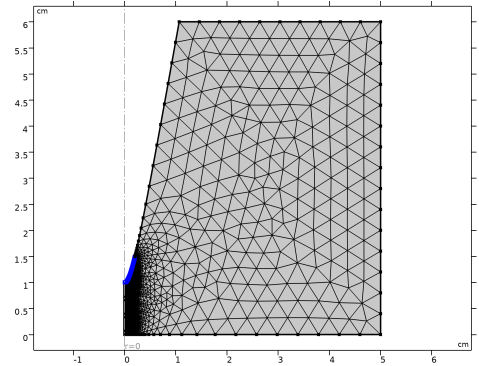
Locate the Element Size Parameters section.
5
Select the Maximum element size checkbox. In the associated text field, type 1/150.
Free Triangular 2
In the Mesh toolbar, click  Free Triangular.
Boundary Layers 1
1
In the Mesh toolbar, click  Boundary Layers.
2
Click the  Zoom Out button in the Graphics toolbar.
3
Click the  Zoom Out button in the Graphics toolbar.
Boundary Layer Properties
1
In the Model Builder window, click Boundary Layer Properties.
2
3
In the Settings window for Boundary Layer Properties, locate the Layers section.
4
In the Number of layers text field, type 3.
5
In the Stretching factor text field, type 1.5.
6
Click  Build All.
7
Click the  Zoom Extents button in the Graphics toolbar.
Study 1
1
In the Model Builder window, click Study 1.
2
In the Settings window for Study, locate the Study Settings section.
3
Clear the Generate default plots checkbox.
Step 2: Time Dependent
1
In the Model Builder window, under Study 1 click Step 2: Time Dependent.
2
In the Settings window for Time Dependent, locate the Study Settings section.
3
From the Time unit list, choose ns.
4
In the Output times text field, type 0 range(1,2,23).
Solution 1 (sol1)
1
In the Study toolbar, click  Show Default Solver.
2
In the Model Builder window, expand the Solution 1 (sol1) node.
3
In the Model Builder window, under Study 1 > Solver Configurations > Solution 1 (sol1) click Time-Dependent Solver 1.
4
In the Settings window for Time-Dependent Solver, click to expand the Time Stepping section.
5
From the Maximum step constraint list, choose Constant.
6
In the Maximum step text field, type 0.025.
7
In the Model Builder window, under Study 1 > Solver Configurations > Solution 1 (sol1) > Time-Dependent Solver 1 click Segregated 1.
8
In the Settings window for Segregated, locate the General section.
9
From the Stabilization and acceleration list, choose Anderson acceleration.
10
Right-click Study 1 > Solver Configurations > Solution 1 (sol1) > Time-Dependent Solver 1 > Segregated 1 and choose Segregated Step.
11
Drag and drop Study  1 > Solver Configurations > Solution 1 (sol1) > Time-Dependent Solver 1 > Segregated 1 > Segregated Step 4below Segregated Step 1.
12
In the Model Builder window, under Study 1 > Solver Configurations > Solution 1 (sol1) > Time-Dependent Solver 1 > Segregated 1 click Segregated Step 1.
13
In the Settings window for Segregated Step, locate the General section.
14
In the Variables list, choose Natural Logarithm of the Number Density Multiplied by 1[cm^3] (comp1.edis.logn_p) and Natural Logarithm of the Number Density Multiplied by 1[cm^3] (comp1.edis.logn_n).
15
Under Variables, click  Delete.
16
Click to expand the Method and Termination section. In the Model Builder window, under Study 1 > Solver Configurations > Solution 1 (sol1) > Time-Dependent Solver 1 > Segregated 1 click Segregated Step 4.
17
In the Settings window for Segregated Step, locate the General section.
18
Under Variables, click  Add.
19
In the Add dialog, in the Variables list, choose Natural Logarithm of the Number Density Multiplied by 1[cm^3] (comp1.edis.logn_n) and Natural Logarithm of the Number Density Multiplied by 1[cm^3] (comp1.edis.logn_p).
20
21
In the Settings window for Segregated Step, locate the Method and Termination section.
22
From the Jacobian update list, choose Once per time step.
23
In the Study toolbar, click  Compute.
Results
Axial Electric Field
1
In the Results toolbar, click  1D Plot Group.
2
In the Settings window for 1D Plot Group, type Axial Electric Field in the Label text field.
Line Graph 1
1
Right-click Axial Electric Field and choose Line Graph.
2
3
In the Settings window for Line Graph, locate the y-Axis Data section.
4
In the Expression text field, type edis.Ez.
5
In the Unit field, type kV/cm.
6
Locate the x-Axis Data section. From the Parameter list, choose Expression.
7
In the Expression text field, type z.
Axial Electric Field
1
In the Model Builder window, click Axial Electric Field.
2
In the Settings window for 1D Plot Group, locate the Legend section.
3
From the Position list, choose Lower left.
Line Graph 1
1
In the Model Builder window, click Line Graph 1.
2
In the Settings window for Line Graph, click to expand the Legends section.
3
Select the Show legends checkbox.
Electron Density at the Axis
1
In the Results toolbar, click  1D Plot Group.
2
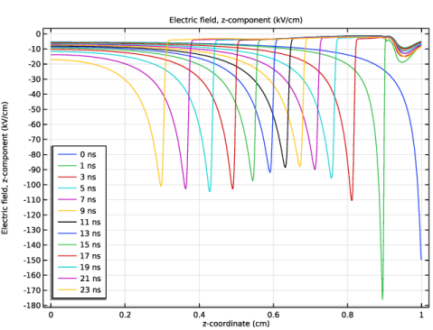
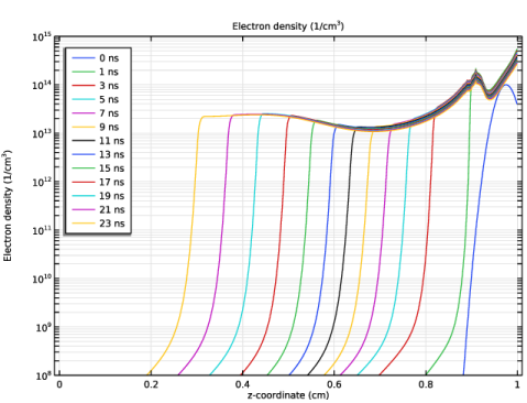
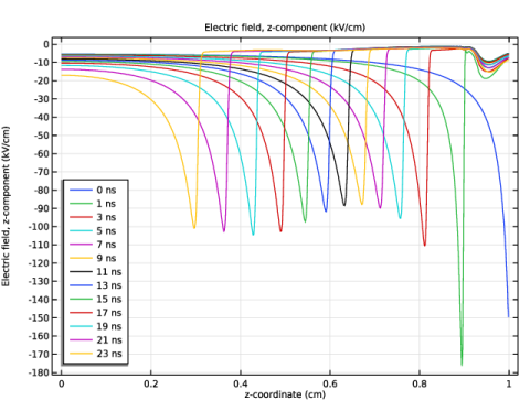
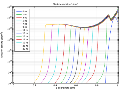
In the Settings window for 1D Plot Group, type Electron Density at the Axis in the Label text field.
Line Graph 1
1
Right-click Electron Density at the Axis and choose Line Graph.
2
3
In the Settings window for Line Graph, locate the y-Axis Data section.
4
In the Expression text field, type edis.n_e.
5
In the Unit field, type 1/cm^3.
6
Locate the x-Axis Data section. From the Parameter list, choose Expression.
7
In the Expression text field, type z.
8
Locate the Legends section. Select the Show legends checkbox.
9
In the Electron Density at the Axis toolbar, click  Plot.
10
Click the  y-Axis Log Scale button in the Graphics toolbar.
Electron Density at the Axis
1
In the Model Builder window, click Electron Density at the Axis.
2
In the Settings window for 1D Plot Group, locate the Axis section.
3
Select the Manual axis limits checkbox.
4
In the y minimum text field, type 1e8.
5
In the y maximum text field, type 1e15.
6
Locate the Legend section. From the Position list, choose Upper left.
7
In the Electron Density at the Axis toolbar, click  Plot.
Mirror 2D 1
In the Results toolbar, click  More Datasets and choose Mirror 2D.
Selection
1
In the Results toolbar, click  Attributes and choose Selection.
2
In the Settings window for Selection, locate the Geometric Entity Selection section.
3
From the Geometric entity level list, choose Domain.
4
2D Plot Group 3
1
In the Results toolbar, click  2D Plot Group.
2
In the Settings window for 2D Plot Group, locate the Data section.
3
From the Dataset list, choose Mirror 2D 1.
4
Locate the Plot Settings section. Clear the Plot dataset edges checkbox.
Surface 1
1
Right-click 2D Plot Group 3 and choose Surface.
2
In the Settings window for Surface, locate the Expression section.
3
In the Expression text field, type edis.normE.
4
In the Unit field, type kV/cm.
Solution Array 1
1
Right-click Surface 1 and choose Solution Array.
2
In the Settings window for Solution Array, locate the Data section.
3
From the Time selection list, choose From list.
4
In the Times (ns) list, choose 5, 11, 17, and 23.
Annotation 1
1
In the Model Builder window, right-click 2D Plot Group 3 and choose Annotation.
2
In the Settings window for Annotation, locate the Coloring and Style section.
3
Clear the Show point checkbox.
4
From the Anchor point list, choose Upper middle.
5
Locate the Annotation section. In the Text text field, type t = eval(t,ns,3) ns.
6
Click to expand the Plot Array section. Select the Manual indexing checkbox.
Solution Array 1
In the Model Builder window, under Results > 2D Plot Group 3 > Surface 1 right-click Solution Array 1 and choose Copy.
Solution Array 1
In the Model Builder window, right-click Annotation 1 and choose Paste Solution Array.
Annotation 1
1
Click the  Zoom Extents button in the Graphics toolbar.
2
In the 2D Plot Group 3 toolbar, click  Plot.
Electric Field
1
In the Model Builder window, under Results click 2D Plot Group 3.
2
In the Settings window for 2D Plot Group, type Electric Field in the Label text field.
3
Click the  Show Grid button in the Graphics toolbar.
4
Click to expand the Title section. From the Title type list, choose Custom.
5
Find the Solution subsection. Clear the Solution checkbox.
6
In the Electric Field toolbar, click  Plot.
7
Click the  Zoom Extents button in the Graphics toolbar.
Electric Field 1
Right-click Electric Field and choose Duplicate.
Surface 1
1
In the Model Builder window, expand the Electric Field 1 node, then click Surface 1.
2
In the Settings window for Surface, locate the Expression section.
3
In the Expression text field, type edis.n_e.
4
In the Unit field, type 1/cm^3.
5
Locate the Coloring and Style section. From the Scale list, choose Logarithmic.
6
From the Color table list, choose Prism.
Electron Density
1
In the Model Builder window, under Results click Electric Field 1.
2
In the Settings window for 2D Plot Group, type Electron Density in the Label text field.
3
In the Electron Density toolbar, click  Plot.
4
Click the  Zoom Extents button in the Graphics toolbar.
Electron Density 1
Right-click Electron Density and choose Duplicate.
Surface 1
1
In the Model Builder window, expand the Electron Density 1 node, then click Surface 1.
2
In the Settings window for Surface, locate the Expression section.
3
In the Expression text field, type edis.Sph.
4
Locate the Coloring and Style section. From the Color table list, choose Magma.
Photoionization Rate
1
In the Model Builder window, under Results click Electron Density 1.
2
In the Settings window for 2D Plot Group, type Photoionization Rate in the Label text field.
3
In the Photoionization Rate toolbar, click  Plot.
4
Click the  Zoom Extents button in the Graphics toolbar.