PDF

Positive Glow Corona Discharge
Introduction
Corona discharges, a prevalent occurrence in both industrial processes and natural phenomena, arise when high voltages are applied to pointed electrodes. These electrodes generate intense electric fields that ionize surrounding gases without causing a complete breakdown across the gap. Typically confined to a localized area, corona discharges manifest as a uniform glow. The characteristics of stable glow corona discharges vary depending on polarity. Positive glow corona, also known as Hermstein’s glow or ultra corona, exhibits a direct current (DC) component overlaid with stable current pulses.
This case study investigates a positive glow corona between coaxial cylindrical electrodes. The electric field dynamics and the concentration of charged particles are determined. The total discharge current, alongside the electronic and ionic current constituents, is computed. The simulated electric field, discharge current, and charge-carrier density are in good agreement with those published in Ref. 1.
Model Definition
The Electric Discharge interface is used to simulate the positive corona. The built-in charge transport model is used:
where
e, p, n denote electrons, positive ions, and negative ions
ni is the number density of the charge carrier (SI unit: 1/m3)
E is the electric field (SI unit: V/m)
zi denotes the carrier charge (SI unit: 1)
μi denotes the carrier mobility (SI unit: m2/(V·s))
wi is the drift velocity in the electric field (SI unit: m/s)
Di is the diffusion coefficient (SI unit: m2/s)
Ri is the reaction rate (SI unit: 1/(m3·s))
α is the ionization coefficient (SI unit: 1/m)
η is the attachment coefficient (SI unit: 1/m)
βep is the electron–ion recombination coefficient (SI unit: m3/s)
βpn is the ion–ion recombination coefficient (SI unit: m3/s)
The above transport equations are fully coupled with Poisson’s equation through the electric field and the space charge:
where e is the elementary charge.
For atmospheric pressure positive discharges, photoionization is critical. This model uses the radiative transfer model for computing photoionization. See Photoionization in the Electric Discharge Module User’s Guide for further details.
where
Sphjdenotes jth photoionization rate component (SI unit: 1/(m3·s))
pp is the partial pressure (default value: 150 Torr)
p is the gas pressure (default value: 760 Torr)
pq is the quenching pressure (default value: 30 Torr)
ξνui is the photoionization parameter (default value: 0.06)
Aj and λj are fitting parameter
Iph is the effective ionization intensity (SI unit: 1/(m3·s))
Sion is the impact ionization rate (SI unit: 1/(m3·s))
Results and Discussion
Figure 1 shows the discharge current as a function of time. Figure 2 plots the distribution of different charge carriers density before and during a current pulse. Figure 3 shows the space charge density distribution at t = 19 μs.
Figure 1: The positive glow corona discharge current and its components due to different charge carriers.
Figure 2: The radial distributions of electron density, positive ion density, and negative ion density at t = 17.4 μs and t = 17.6 μs.
Figure 3: The distribution of space charge density at t = 19 μs.
References
1. R. Morrow, “The theory of positive glow corona,” J. Phys. D: Appl. Phys., vol. 30, no. 22,p. 3099, 1997.
Application Library path: Electric_Discharge_Module/Corona_Discharges/positive_glow_corona
Modeling Instructions
From the File menu, choose New.
New
In the New window, click  Model Wizard.
Model Wizard
1
In the Model Wizard window, click  1D Axisymmetric.
2
In the Select Physics tree, select Electric Discharge > Electric Discharge (edis).
3
Click Add.
4
Click  Study.
5
In the Select Study tree, select Preset Studies for Selected Physics Interfaces > Time Dependent with Initialization.
6
Global Definitions
Parameters 1
1
In the Model Builder window, under Global Definitions click Parameters 1.
2
In the Settings window for Parameters, locate the Parameters section.
3
Ramp 1 (rm1)
1
In the Home toolbar, click  Functions and choose Global > Ramp.
2
In the Settings window for Ramp, locate the Parameters section.
3
In the Slope text field, type 3.
4
Select the Cutoff checkbox. In the associated text field, type 30.
5
Click to expand the Smoothing section.
6
Select the Size of transition zone at cutoff checkbox. In the associated text field, type 1.
Geometry 1
1
In the Model Builder window, expand the Component 1 (comp1) > Geometry 1 node, then click Geometry 1.
2
In the Settings window for Geometry, locate the Units section.
3
From the Length unit list, choose cm.
Interval 1 (i1)
1
Right-click Geometry 1 and choose Interval.
2
In the Settings window for Interval, locate the Interval section.
3
Electric Discharge (edis)
Gas 1
In the Model Builder window, under Component 1 (comp1) > Electric Discharge (edis) click Gas 1.
Electrode 1
1
In the Physics toolbar, click  Attributes and choose Electrode.
2
3
In the Settings window for Electrode, locate the Charge Transport section.
4
From the Boundary condition for electrons list, choose Number density.
5
From the Boundary condition for negative ions list, choose Number density.
Gas 1
In the Model Builder window, click Gas 1.
Electrode 2
1
In the Physics toolbar, click  Attributes and choose Electrode.
2
3
In the Settings window for Electrode, locate the Terminal section.
4
In the V0 text field, type V0.
5
Locate the Charge Transport section. From the Boundary condition for positive ions list, choose Number density.
Gas 1
In the Model Builder window, click Gas 1.
Photoionization 1
In the Physics toolbar, click  Attributes and choose Photoionization.
Add Material
1
In the Materials toolbar, click  Add Material to open the Add Material window.
2
Go to the Add Material window.
3
In the tree, select Electric Discharge > Gases > Air > Air [Morrow and Lowke, 1997].
4
Right-click and choose Add to Component 1 (comp1).
5
In the Materials toolbar, click  Add Material to close the Add Material window.
Mesh 1
Edge 1
In the Mesh toolbar, click  Edge.
Distribution 1
1
In the Model Builder window, right-click Edge 1 and choose Distribution.
2
In the Settings window for Distribution, locate the Distribution section.
3
From the Distribution type list, choose Predefined.
4
In the Number of elements text field, type 300.
5
In the Element ratio text field, type 10.
6
Click  Build All.
Definitions
Domain Probe 1 (dom1)
1
In the Model Builder window, expand the Component 1 (comp1) > Definitions node.
2
Right-click Definitions and choose Probes > Domain Probe.
3
In the Settings window for Domain Probe, locate the Probe Type section.
4
From the Type list, choose Integral.
5
Locate the Expression section. In the Expression text field, type abs(edis.Jc_er*edis.Er/V0).
6
In the Table and plot unit field, type mA/m.
7
In the Variable name text field, type i_e.
8
Locate the Expression section.
9
Select the Description checkbox. In the associated text field, type Electron Current.
Domain Probe 2 (dom2)
1
Right-click Domain Probe 1 (i_e) and choose Duplicate.
2
In the Settings window for Domain Probe, type i_p in the Variable name text field.
3
Locate the Expression section. In the Expression text field, type abs(edis.Jc_pr*edis.Er/V0).
4
In the Description text field, type Positive Ion Current.
Domain Probe 3 (dom3)
1
Right-click Domain Probe 2 (i_p) and choose Duplicate.
2
In the Settings window for Domain Probe, type i_n in the Variable name text field.
3
Locate the Expression section. In the Expression text field, type abs(edis.Jc_nr*edis.Er/V0).
4
In the Description text field, type Negative Ion Current.
Domain Probe 4 (dom4)
1
Right-click Domain Probe 3 (i_n) and choose Duplicate.
2
In the Settings window for Domain Probe, type i_d in the Variable name text field.
3
Locate the Expression section. In the Expression text field, type edis.Jdr*edis.Er/V0.
4
In the Description text field, type Displacement Current.
Global Variable Probe 1 (var1)
1
In the Definitions toolbar, click  Probes and choose Global Variable Probe.
2
In the Settings window for Global Variable Probe, type i_dom in the Variable name text field.
3
Locate the Expression section. In the Expression text field, type i_e+i_p+i_n+i_d.
4
In the Table and plot unit field, type mA/m.
5
Select the Description checkbox. In the associated text field, type Total Current, Domain.
Global Variable Probe 2 (var2)
1
In the Definitions toolbar, click  Probes and choose Global Variable Probe.
2
In the Settings window for Global Variable Probe, type i_bnd in the Variable name text field.
3
Locate the Expression section. In the Expression text field, type edis.I0_1/edis.d.
4
In the Table and plot unit field, type mA/m.
5
Select the Description checkbox. In the associated text field, type Total Current, Boundary.
Study 1
Step 2: Time Dependent
1
In the Model Builder window, under Study 1 click Step 2: Time Dependent.
2
In the Settings window for Time Dependent, locate the Study Settings section.
3
From the Time unit list, choose µs.
4
In the Output times text field, type range(5,2,15) range(17,0.2,19).
Solution 1 (sol1)
1
In the Study toolbar, click  Show Default Solver.
2
In the Model Builder window, click Study 1.
3
In the Settings window for Study, locate the Study Settings section.
4
Clear the Generate default plots checkbox.
5
In the Model Builder window, expand the Solution 1 (sol1) node, then click Time-Dependent Solver 1.
6
In the Settings window for Time-Dependent Solver, click to expand the Time Stepping section.
7
From the Maximum step constraint list, choose Constant.
8
In the Maximum step text field, type 3[ns].
9
In the Study toolbar, click  Compute.
Results
Probe Plot Group 1
1
In the Model Builder window, under Results click Probe Plot Group 1.
2
In the Settings window for 1D Plot Group, locate the Plot Settings section.
3
Select the y-axis label checkbox. In the associated text field, type Current, mA/m.
Probe Table Graph 1
1
In the Model Builder window, expand the Probe Plot Group 1 node, then click Probe Table Graph 1.
2
In the Settings window for Table Graph, locate the Coloring and Style section.
3
Find the Line markers subsection. From the Marker list, choose Cycle.
4
In the Probe Plot Group 1 toolbar, click  Plot.
1D Plot Group 2
1
In the Results toolbar, click  1D Plot Group.
2
In the Settings window for 1D Plot Group, locate the Data section.
3
From the Dataset list, choose None.
Line Graph 1
1
Right-click 1D Plot Group 2 and choose Line Graph.
2
In the Settings window for Line Graph, locate the Data section.
3
From the Dataset list, choose Study 1/Solution 1 (sol1).
4
From the Time selection list, choose From list.
5
In the Times (µs) list, choose 17.4 and 17.6.
6
7
Locate the y-Axis Data section. In the Expression text field, type edis.n_e.
8
In the Unit field, type 1/cm^3.
9
Click to expand the Coloring and Style section. Find the Line style subsection. From the Line list, choose Dotted.
10
Find the Line markers subsection. From the Marker list, choose Cycle (reset).
11
From the Positioning list, choose Interpolated.
12
Click to expand the Legends section. Select the Show legends checkbox.
13
Find the Include subsection. Select the Description checkbox.
14
In the 1D Plot Group 2 toolbar, click  Plot.
Line Graph 2
1
Right-click Line Graph 1 and choose Duplicate.
2
In the Settings window for Line Graph, locate the y-Axis Data section.
3
In the Expression text field, type edis.n_p.
4
Locate the Coloring and Style section. Find the Line style subsection. From the Line list, choose Solid.
Line Graph 3
1
Right-click Line Graph 2 and choose Duplicate.
2
In the Settings window for Line Graph, locate the y-Axis Data section.
3
In the Expression text field, type edis.n_n.
4
Locate the Coloring and Style section. Find the Line style subsection. From the Line list, choose Dashed.
1D Plot Group 2
1
In the Model Builder window, click 1D Plot Group 2.
2
In the Settings window for 1D Plot Group, locate the Plot Settings section.
3
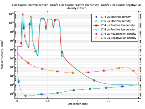
Select the y-axis label checkbox. In the associated text field, type Number Density, 1/cm<sup>3</sup>.
4
Click the  y-Axis Log Scale button in the Graphics toolbar.
5
In the 1D Plot Group 2 toolbar, click  Plot.
Revolution 1D 1
1
In the Model Builder window, expand the Results > Datasets node.
2
Right-click Results > Datasets and choose Revolution 1D.
2D Plot Group 3
In the Results toolbar, click  2D Plot Group.
Surface 1
1
In the Model Builder window, right-click 2D Plot Group 3 and choose Surface.
2
In the Settings window for Surface, locate the Expression section.
3
From the Unit list, choose µC/m^3.
4
In the 2D Plot Group 3 toolbar, click  Plot.