|
|
|

|
•
|
|
•
|
|
•
|
E is the electric field (SI unit: V/m)
|
|
•
|
zi denotes the carrier charge (SI unit: 1)
|
|
•
|
|
•
|
wi is the drift velocity in the electric field (SI unit: m/s)
|
|
•
|
|
•
|
|
•
|
α is the ionization coefficient (SI unit: 1/m)
|
|
•
|
η is the attachment coefficient (SI unit: 1/m)
|
|
•
|
|
•
|

|
1
|
|
2
|
|
3
|
Click Add.
|
|
4
|
Click
|
|
5
|
In the Select Study tree, select Preset Studies for Selected Physics Interfaces > Time Dependent with Initialization.
|
|
6
|
Click
|
|
1
|
|
2
|
|
1
|
|
2
|
|
3
|
|
1
|
|
2
|
|
1
|
|
2
|
|
3
|
|
4
|
|
5
|
Select the Layers to the left checkbox.
|
|
7
|
Click
|
|
1
|
|
2
|
|
3
|
|
4
|
|
5
|
|
6
|
Click
|
|
1
|
|
2
|
On the object pc1, select Point 2 only.
|
|
3
|
|
4
|
|
5
|
On the object r1, select Point 4 only.
|
|
6
|
Click
|
|
1
|
|
2
|
On the object ls1, select Point 2 only.
|
|
3
|
|
4
|
|
5
|
On the object pc1, select Point 1 only.
|
|
6
|
|
7
|
Click
|
|
1
|
|
2
|
|
3
|
|
1
|
|
2
|
|
3
|
|
4
|
|
5
|
Select the object csol1 only.
|
|
1
|
In the Model Builder window, under Component 1 (comp1) > Geometry 1 right-click Parametric Curve 1 (pc1) and choose Duplicate.
|
|
2
|
|
3
|
|
4
|
|
1
|
|
2
|
|
3
|
|
4
|
Click
|
|
5
|
|
1
|
|
2
|
|
3
|
|
4
|
Click OK.
|
|
5
|
|
6
|
In the Settings window for Electric Discharge, click to expand the Consistent Stabilization section.
|
|
7
|
Clear the Streamline diffusion checkbox.
|
|
8
|
|
9
|
|
10
|
|
1
|
|
3
|
|
4
|
|
1
|
|
2
|
|
3
|
|
4
|
|
5
|
|
6
|
|
1
|
|
2
|
|
3
|
|
4
|
|
5
|
|
1
|
|
2
|
In the Settings window for Dielectric Interface, Bulk Transport, locate the Charge Transport section.
|
|
3
|
|
1
|
|
3
|
|
4
|
|
5
|
Locate the Charge Transport section. From the Boundary condition for electrons list, choose Surface emission.
|
|
6
|
|
7
|
|
8
|
Locate the Surface Emission section. Find the Surface emission mechanisms subsection. Select the Secondary electron emission checkbox.
|
|
1
|
|
1
|
|
2
|
Go to the Add Material window.
|
|
3
|
|
4
|
Right-click and choose Add to Component 1 (comp1).
|
|
5
|
|
1
|
In the Model Builder window, under Component 1 (comp1) right-click Materials and choose Blank Material.
|
|
2
|
|
4
|
Locate the Material Contents section. In the table, enter the following settings:
|
|
1
|
|
3
|
|
4
|
Locate the Material Contents section. In the table, enter the following settings:
|
|
1
|
|
2
|
|
3
|
From the list, choose User-controlled mesh.
|
|
1
|
|
2
|
Drag and drop below Size.
|
|
3
|
|
4
|
|
1
|
|
3
|
|
4
|
|
5
|
|
6
|
|
1
|
|
3
|
|
4
|
|
5
|
|
6
|
|
7
|
Select the Reverse direction checkbox.
|
|
1
|
|
3
|
|
4
|
|
5
|
|
6
|
|
7
|
Select the Reverse direction checkbox.
|
|
1
|
|
2
|
|
3
|
|
5
|
|
6
|
Locate the Element Size Parameters section.
|
|
7
|
|
8
|
|
1
|
|
2
|
|
3
|
|
5
|
|
6
|
Locate the Element Size Parameters section.
|
|
7
|
|
1
|
|
3
|
|
4
|
|
5
|
|
6
|
|
7
|
Click
|
|
1
|
|
2
|
|
3
|
Click
|
|
4
|
|
5
|
Click OK.
|
|
6
|
|
7
|
|
8
|
|
9
|
|
10
|
|
11
|
|
1
|
|
2
|
|
3
|
|
4
|
|
5
|
|
1
|
|
2
|
|
3
|
|
4
|
|
5
|
|
6
|
|
7
|
Clear the Generate default plots checkbox.
|
|
1
|
|
2
|
|
3
|
In the Model Builder window, expand the Study 1 > Solver Configurations > Solution 1 (sol1) > Time-Dependent Solver 1 node.
|
|
4
|
In the Model Builder window, under Study 1 > Solver Configurations > Solution 1 (sol1) > Time-Dependent Solver 1 click Segregated 1.
|
|
5
|
|
6
|
|
7
|
In the Model Builder window, under Study 1 > Solver Configurations > Solution 1 (sol1) > Time-Dependent Solver 1 > Segregated 1 click Segregated Step 1.
|
|
8
|
|
9
|
|
10
|
In the Model Builder window, under Study 1 > Solver Configurations > Solution 1 (sol1) > Time-Dependent Solver 1 > Segregated 1 click Segregated Step 2.
|
|
11
|
|
12
|
|
13
|
|
1
|
|
2
|
|
3
|
|
4
|
|
5
|
|
1
|
|
2
|
|
3
|
|
4
|
|
5
|
|
6
|
|
7
|
|
8
|
|
1
|
|
2
|
|
3
|
|
4
|
|
5
|
|
6
|
|
8
|
|
9
|
|
10
|
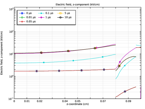
Click to expand the Coloring and Style section. Find the Line markers subsection. From the Marker list, choose Cycle.
|
|
11
|
|
12
|
|
13
|
|
1
|
|
2
|
|
1
|
|
2
|
|
3
|
|
4
|
|
1
|
|
2
|
|
3
|
|
4
|
|
5
|
|
6
|
Click
|
|
8
|
|
9
|
Locate the Coloring and Style section. Find the Line markers subsection. In the Number text field, type 8.
|
|
1
|
|
2
|
|
3
|
|
4
|
|
5
|
|
6
|
|
1
|
|
2
|
|
1
|
|
2
|
|
3
|
|
1
|
|
2
|
|
3
|
|
4
|
|
5
|
|
1
|
|
2
|
|
3
|
|
4
|
|
5
|
|
6
|
Click
|
|
1
|
|
2
|
|
3
|
|
4
|
|
5
|
|
6
|
|
1
|
|
2
|
|
1
|
|
2
|
|
3
|
Select the Cutoff checkbox.
|
|
1
|
In the Model Builder window, expand the Component 1 (comp1) > Electric Discharge 2 (edis2) > Gas 1 node, then click Electrode 1.
|
|
2
|
|
3
|
|
4
|
Locate the Charge Transport section. From the Boundary condition for electrons list, choose Number density.
|
|
5
|
|
1
|
|
2
|
In the Settings window for Dielectric Interface, Bulk Transport, locate the Charge Transport section.
|
|
3
|
|
1
|
In the Model Builder window, under Component 1 (comp1) > Definitions right-click Global Variable Probe 1 (i0) and choose Duplicate.
|
|
2
|
|
3
|
|
4
|
|
5
|
Click
|
|
1
|
|
2
|
|
1
|
In the Model Builder window, under Study 1, Fast Charging click Step 1: Electrostatics Initialization.
|
|
2
|
In the Settings window for Electrostatics Initialization, locate the Physics and Variables Selection section.
|
|
3
|
Select the Modify model configuration for study step checkbox.
|
|
4
|
|
5
|
Right-click and choose Disable in Model.
|
|
1
|
|
2
|
|
3
|
Select the Modify model configuration for study step checkbox.
|
|
4
|
|
5
|
Right-click and choose Disable in Model.
|
|
6
|
|
7
|
|
8
|
|
1
|
|
2
|
Go to the Add Study window.
|
|
3
|
Find the Studies subsection. In the Select Study tree, select Preset Studies for Selected Physics Interfaces > Time Dependent with Initialization.
|
|
4
|
Click the Add Study button in the window toolbar.
|
|
1
|
In the Settings window for Electrostatics Initialization, locate the Physics and Variables Selection section.
|
|
2
|
In the Solve for column of the table, under Component 1 (comp1), clear the checkbox for Electric Discharge (edis).
|
|
1
|
|
2
|
|
3
|
In the Solve for column of the table, under Component 1 (comp1), clear the checkbox for Electric Discharge (edis).
|
|
4
|
|
5
|
|
6
|
|
7
|
|
8
|
|
1
|
In the Model Builder window, expand the Component 1 (comp1) > Meshes > Mesh 2 > Mapped 1 node, then click Distribution 1.
|
|
2
|
|
3
|
|
1
|
|
2
|
|
3
|
|
1
|
In the Model Builder window, expand the Component 1 (comp1) > Meshes > Mesh 2 > Free Triangular 1 node, then click Size 1.
|
|
2
|
|
3
|
|
1
|
In the Model Builder window, expand the Component 1 (comp1) > Meshes > Mesh 2 > Boundary Layers 1 node, then click Component 1 (comp1) > Meshes > Mesh 2 > Free Triangular 1 > Size 2.
|
|
2
|
|
3
|
|
1
|
In the Model Builder window, under Component 1 (comp1) > Meshes > Mesh 2 > Boundary Layers 1 right-click Boundary Layer Properties and choose Build All.
|
|
2
|
|
1
|
|
2
|
In the Settings window for Electrostatics Initialization, click to expand the Mesh Selection section.
|
|
1
|
|
2
|
|
4
|
|
5
|
|
6
|
|
7
|
|
1
|
|
2
|
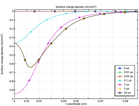
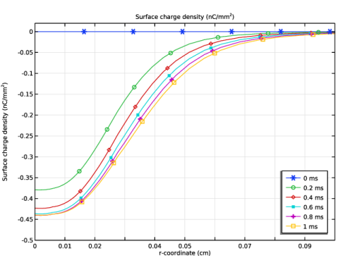
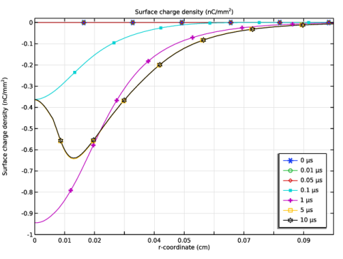
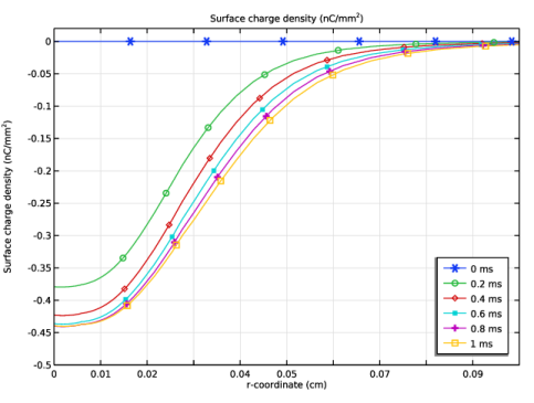
In the Settings window for 1D Plot Group, type Surface Charge Density, Slow Charging in the Label text field.
|
|
3
|
|
4
|
|
1
|
In the Model Builder window, expand the Surface Charge Density, Slow Charging node, then click Line Graph 1.
|
|
2
|
|
3
|
|
4
|