|
|
|

|
•
|
|
•
|
|
•
|
E is the electric field (SI unit: V/m)
|
|
•
|
zi denotes the carrier charge (SI unit: 1)
|
|
•
|
|
•
|
wi is the drift velocity in the electric field (SI unit: m/s)
|
|
•
|
|
•
|
|
•
|
α is the ionization coefficient (SI unit: 1/m)
|
|
•
|
η is the attachment coefficient (SI unit: 1/m)
|
|
•
|
|
•
|

|
1
|
|
2
|
|
3
|
Click Add.
|
|
4
|
Click
|
|
5
|
In the Select Study tree, select Preset Studies for Selected Physics Interfaces > Time Dependent with Initialization.
|
|
6
|
Click
|
|
1
|
|
2
|
|
3
|
|
1
|
|
2
|
|
1
|
|
2
|
|
4
|
|
1
|
|
2
|
|
3
|
Select the Solid checkbox.
|
|
1
|
|
3
|
|
4
|
|
5
|
Locate the Constitutive Relation D-E section. From the εr list, choose User defined. In the associated text field, type 3.5.
|
|
1
|
Go to the Add Material window.
|
|
2
|
|
3
|
Right-click and choose Add to Component 1 (comp1).
|
|
1
|
In the Model Builder window, under Component 1 (comp1) > Materials click Air [Morrow and Lowke, 1997] (mat1).
|
|
2
|
|
3
|
|
4
|
Click
|
|
1
|
|
3
|
|
4
|
|
1
|
|
1
|
|
2
|
|
3
|
From the list, choose User-controlled mesh.
|
|
1
|
|
3
|
|
4
|
|
5
|
|
6
|
|
7
|
Select the Symmetric distribution checkbox.
|
|
1
|
|
3
|
|
4
|
|
5
|
|
1
|
|
2
|
|
3
|
|
1
|
|
2
|
|
3
|
|
1
|
|
2
|
|
3
|
Click
|
|
5
|
|
6
|
|
7
|
Clear the Generate default plots checkbox.
|
|
8
|
|
1
|
|
2
|
|
3
|
|
4
|
|
5
|
Locate the y-Axis Data section. In the table, enter the following settings:
|
|
6
|
|
1
|
|
2
|
|
3
|
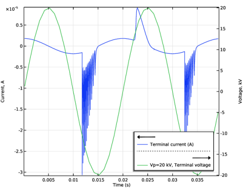
Select the Two y-axes checkbox.
|
|
4
|
|
5
|
|
6
|
|
7
|
|
8
|
|
9
|
|
1
|
|
2
|
|
1
|
|
3
|
|
4
|
|
5
|
|
1
|
|
2
|
|
3
|
|
4
|
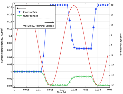
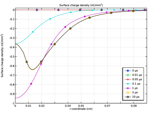
Select the y-axis label checkbox. In the associated text field, type Surface charge density, nC/mm<sup>2</sup>.
|
|
5
|
Select the Secondary y-axis label checkbox.
|
|
1
|
|
2
|
|
3
|
Select the Show legends checkbox.
|
|
4
|
|
6
|
Click to expand the Coloring and Style section. Find the Line markers subsection. From the Marker list, choose Cycle.
|
|
1
|
|
2
|
|
3
|
|
4
|