PDF

Orange Battery
Introduction
This tutorial model serves as an introduction to electrochemistry modeling in COMSOL Multiphysics. The example simulates the currents and the concentration of dissolved metal ions in a battery (corrosion cell) made from an orange and two metal nails.
Figure 1: Modeled geometry. Orange and two metal nails. (Due to the high conductivity of the metal nails, only the orange pulp is included in the computational domain.)
This type of battery is commonly used in chemistry class demonstrations. Instead of an orange, lemons or potatoes can also be used.
Model Definition
The citric acid and various other ions in the orange serves as electrolyte, and using nails of different metals as electrodes creates a galvanic potential over the cell.
In this example, a zinc nail is used as one of the electrodes, giving rise to the following electrode reaction:
The other nail consists of copper, and here hydrogen evolution is assumed to take place:
Eeq,0 above denotes the equilibrium potentials at standard conditions versus a standard hydrogen electrode (SHE). In the model, the equilibrium potentials are corrected for the pH and zinc concentration of the orange pulp using the Nernst equation.
The model for the currents in the orange and electrodes is set up using the Secondary Current Distribution interface. The electrolyte current in the orange is thereby solved for by Ohm’s law. The conductivity of the metal nails is so high that the electrode domains are not included in the model, instead boundary conditions on the nail surfaces are used to set the nail potentials. One nail is grounded, and the other one is set to a cell voltage to comply with a total current condition. This would correspond to a situation where the cell is controlled galvanostatically, for instance, by the use of a potentiostat.
Butler–Volmer type expressions, with concentration-dependent exchange current density for the zinc reaction, are used for the electrode kinetics on the surface of the nails within the orange.
The initial values electrolyte potential is set to correspond to the potential of a cell at open circuit (that is, no activation potential). Following the definition of the overpotential:
the initial value becomes:
In an extension of the model, the transport of the dissolved zinc ions in the orange from the zinc electrode reaction is modeled by the Transport of Diluted Species interface in a time-dependent simulation. This assumes that the zinc ion transport can be described by diffusion according for Fick’s law. In addition, the zinc electrode kinetics are modified to be dependent on the zinc concentration, which increases in the orange as more and more zinc is dissolved.
The cell current is set to a constant value of 1 mA, and the zinc concentration is set to 0.001 mol/m3 at the start of the simulation. All boundaries except the zinc electrode are insulated.
Results and Discussion
Figure 2 shows the potential field in the orange. The potential decreases as the current flows from the zinc electrode (left) to the upper electrode (right). The main part of the cell voltage loss is due to ohmic losses in the electrolyte.
The performance of the battery could probably be increased by using an electrolyte of higher conductivity (for example, a lemon instead of an orange) or by decreasing the distance between the nails.
Figure 2: Potential field in the electrolyte at t = 0.
Figure 3 shows a polarization plot as the total current of the battery increases from 0 to 1 mA. The large change in cell voltage seen at low currents is due to overpotential losses at the zinc electrode. Increasing the area of the zinc electrode would decrease this effect.
Figure 3: Polarization plot for the initial concentrations.
Figure 4 shows an isosurface for the 0.2 mol/m3 concentration level of zinc ions after running the battery for five minutes. Figure 5 shows how far the 0.2 mol/m3 isosurface level has reached after one hour.
Figure 4: 0.2 mol/m3 zinc concentration isosurface after five minutes.
Figure 5: 0.2 mol/m3 zinc concentration isosurface after one hour.
Figure 6 shows how the cell voltage evolves with time. Due to the increase of zinc ions at the zinc nail electrode, the battery voltage decreases for a constant current.
Figure 6: Cell voltage versus time.
Suggested Exercises and Extensions of the Model
Change the radius of the nails, and the value of the electrolyte conductivity, and investigate how this affects the polarization plot.
The proton concentration is not included in the model. Add the proton concentration under Dependent Variables on the Transport of Diluted Species node and couple the flux of protons on the copper surface by using an Electrode Surface Coupling node. In this manner, the change in pH of the cell can be monitored.
The dissolved zinc ions may form a layer of zinc hydroxide on the zinc surface, giving rise to an additional potential drop. You can use the Film Resistance section on the Electrode Surface node to include this potential drop. The value of the film resistance could, for instance, be a function of the zinc ion concentration variable in the pulp. Alternatively, you can add a Surface Reactions interface to model the buildup of the surface concentration of zinc hydroxide.
Application Library path: Electrodeposition_Module/General_Electrochemistry/orange_battery
Modeling Instructions
From the File menu, choose New.
New
In the New window, click  Model Wizard.
Model Wizard
1
In the Model Wizard window, click  3D.
2
In the Select Physics tree, select Electrochemistry > Primary and Secondary Current Distribution > Secondary Current Distribution (cd).
3
Click Add.
4
Click  Study.
5
In the Select Study tree, select General Studies > Stationary.
6
Geometry 1
Start by drawing the geometry; one sphere (the orange) and two cylinders (the metal nails).
Sphere 1 (sph1)
1
In the Geometry toolbar, click  Sphere.
2
In the Settings window for Sphere, locate the Size section.
3
In the Radius text field, type 5e-2.
Zinc nail
1
In the Geometry toolbar, click  Cylinder.
2
In the Settings window for Cylinder, type Zinc nail in the Label text field.
3
Locate the Size and Shape section. In the Radius text field, type 2e-3.
4
In the Height text field, type 5e-2.
5
Locate the Position section. In the x text field, type -2e-2.
6
In the z text field, type 2e-2.
By enabling Resulting objects selection you can easily select all boundaries of the nail later on when setting up the physics.
7
Locate the Selections of Resulting Entities section. Select the Resulting objects selection checkbox.
8
From the Show in physics list, choose All levels.
Copper nail
Duplicate the cylinder and change the x position to draw the second nail, as follows:
1
Right-click Zinc nail and choose Duplicate.
2
In the Settings window for Cylinder, type Copper nail in the Label text field.
3
Locate the Position section. In the x text field, type 2e-2.
4
In the Geometry toolbar, click  Build All.
Global Definitions
Load some global parameters from a file. These will be used in multiple places in the model.
Parameters 1
1
In the Model Builder window, under Global Definitions click Parameters 1.
2
In the Settings window for Parameters, locate the Parameters section.
3
Click  Load from File.
4
Definitions
Load also some variable definitions from a file.
Variables 1
1
In the Model Builder window, under Component 1 (comp1) right-click Definitions and choose Variables.
2
In the Settings window for Variables, locate the Variables section.
3
Click  Load from File.
4
Secondary Current Distribution (cd)
Now, start setting up the current distribution model.
Change the selection of the entire physics interface to the orange domain only.
1
In the Model Builder window, under Component 1 (comp1) click Secondary Current Distribution (cd).
2
Also create a selection for the orange domain. This will help if the geometry needs to be changed in the future. Selections is generally a convenient way to group different parts of the geometry together.
3
In the Settings window for Secondary Current Distribution, locate the Domain Selection section.
4
Click  Create Selection.
5
In the Create Selection dialog, type Orange in the Selection name text field.
6
Electrolyte 1
An Electrolyte node has already been added to the model by default. The selection is locked to all selected domains of the physics interface, which in this case is the orange only. Set the electrolyte conductivity.
1
In the Model Builder window, under Component 1 (comp1) > Secondary Current Distribution (cd) click Electrolyte 1.
2
In the Settings window for Electrolyte, locate the Electrolyte section.
3
From the σl list, choose User defined. In the associated text field, type sigma.
Electrode Surface 1
Use Electrode Surface nodes to define both a metal electrode potential and an electrode-electrolyte interface. Use a Butler-Volmer expression for the zinc electrode. The hydrogen kinetics are assumed to be very fast so that a linearized Butler-Volmer expression is applicable.
1
In the Physics toolbar, click  Boundaries and choose Electrode Surface.
2
In the Settings window for Electrode Surface, locate the Boundary Selection section.
3
From the Selection list, choose Zinc nail.
Enable transparency and inspect the active boundaries in the graphics window.
4
Click the  Transparency button in the Graphics toolbar.
Electrode Reaction 1
1
In the Model Builder window, click Electrode Reaction 1.
2
In the Settings window for Electrode Reaction, locate the Equilibrium Potential section.
3
From the Eeq list, choose Nernst equation.
4
In the Eeq,ref(T) text field, type Eeqref_Zn.
5
In the CO text field, type c_Zn2/c_ref.
6
Locate the Stoichiometric Coefficients section. In the n text field, type 2.
7
Locate the Electrode Kinetics section. From the Kinetics expression type list, choose Butler–Volmer.
8
From the Exchange current density type list, choose From Nernst Equation.
9
In the i0,ref(T) text field, type i0ref_Zn.
10
In the αa text field, type alpha_a_Zn.
Electrode Surface 2
Now define the copper electrode in a similar way. First add a parameter for the total current. This parameter will also be used in the study to perform a galvanic polarization sweep over the cell.
1
In the Physics toolbar, click  Boundaries and choose Electrode Surface.
2
In the Settings window for Electrode Surface, locate the Boundary Selection section.
3
From the Selection list, choose Copper nail.
4
Locate the Electrode Phase Potential Condition section. From the Electrode phase potential condition list, choose Total current.
5
In the Il,total text field, type -i_app.
Electrode Reaction 1
1
In the Model Builder window, click Electrode Reaction 1.
2
In the Settings window for Electrode Reaction, locate the Equilibrium Potential section.
3
From the Eeq list, choose Nernst equation.
4
In the CO text field, type c_H0/c_ref.
5
Locate the Electrode Kinetics section. In the i0 text field, type i0_H2.
Initial Values 1
We are using nonlinear kinetics in the model. Provide an initial value for the electrolyte potential in order to reduce solver time and improve convergence. As a rule of thumb one can often use the negative of the equilibrium potential of the grounded electrode as initial value for the electrolyte potential.
1
In the Model Builder window, under Component 1 (comp1) > Secondary Current Distribution (cd) click Initial Values 1.
2
In the Settings window for Initial Values, locate the Initial Values section.
3
In the phil text field, type -E_eq_Zn0.
Global Definitions
Default Model Inputs
Set up the temperature value used in the entire model.
1
In the Model Builder window, under Global Definitions click Default Model Inputs.
2
In the Settings window for Default Model Inputs, locate the Browse Model Inputs section.
3
In the tree, select General > Temperature (K) - minput.T.
4
Find the Expression for remaining selection subsection. In the Temperature text field, type T.
Mesh 1
1
In the Model Builder window, under Component 1 (comp1) click Mesh 1.
2
In the Settings window for Mesh, locate the Physics-Controlled Mesh section.
3
From the Element size list, choose Coarse.
Study 1
Since we are using the default mesh settings, the model is now ready for solving.
1
In the Study toolbar, click  Compute.
Results
Electrolyte Potential (cd)
Plots of the electrolyte potentials are created by default.
Use an isosurface for visualizing the potential field in the electrolyte.
Potential Isosurface
1
In the Results toolbar, click  3D Plot Group.
2
In the Settings window for 3D Plot Group, type Potential Isosurface in the Label text field.
Isosurface 1
1
Right-click Potential Isosurface and choose Isosurface.
2
In the Settings window for Isosurface, locate the Levels section.
3
In the Total levels text field, type 25.
4
Click the  Zoom Extents button in the Graphics toolbar.
5
In the Potential Isosurface toolbar, click  Plot.
Study 1
Step 1: Stationary
Now use an Auxiliary Sweep to solve over a range of cell currents in order to create a polarization plot.
1
In the Model Builder window, under Study 1 click Step 1: Stationary.
2
In the Settings window for Stationary, click to expand the Study Extensions section.
3
Select the Auxiliary sweep checkbox.
4
5
6
In the Study toolbar, click  Compute.
Results
Create a polarization plot as follows:
Polarization Plot
1
In the Results toolbar, click  1D Plot Group.
2
In the Settings window for 1D Plot Group, type Polarization Plot in the Label text field.
3
Click to expand the Title section. From the Title type list, choose None.
4
Locate the Plot Settings section.
5
Select the y-axis label checkbox. In the associated text field, type Cell voltage (V).
6
Locate the Legend section. Clear the Show legends checkbox.
Global 1
1
Right-click Polarization Plot and choose Global.
2
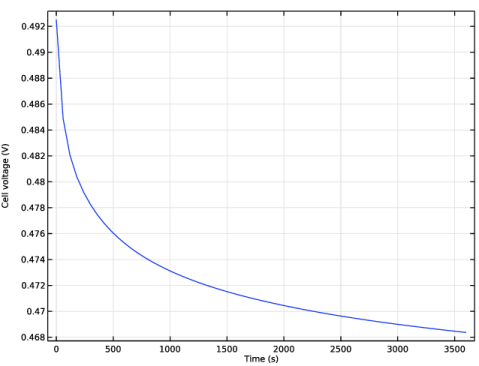
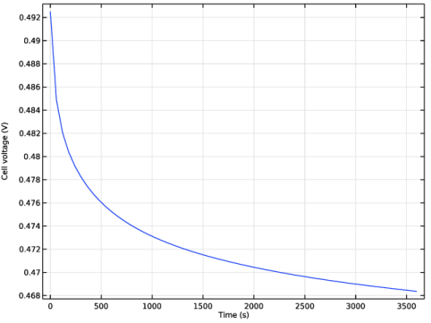
In the Settings window for Global, click Replace Expression in the upper-right corner of the y-Axis Data section. From the menu, choose Component 1 (comp1) > Secondary Current Distribution > cd.phis_es2 - Electric potential - V.
3
In the Polarization Plot toolbar, click  Plot.
Component 1 (comp1)
Now, extend the model to investigate the battery voltage over time at a certain load current. Start by adding a physics interface to handle the mass transport of zinc ions.
Add Physics
1
In the Home toolbar, click  Add Physics to open the Add Physics window.
2
Go to the Add Physics window.
3
In the tree, select Chemical Species Transport > Transport of Diluted Species (tds).
4
Click the Add to Component 1 button in the window toolbar.
5
In the Home toolbar, click  Add Physics to close the Add Physics window.
Transport of Diluted Species (tds)
1
In the Settings window for Transport of Diluted Species, locate the Domain Selection section.
2
From the Selection list, choose Orange.
Because the orange pulp is stationary, convection does not need to be included in the model.
3
Locate the Transport Mechanisms section. Clear the Convection checkbox.
Due to the presence of a lot of other ions in the pulp, acting as supporting electrolyte, we assume the potential gradients to be small and hence also ignore the effect of migrative transport of the zinc ions.
Electrode Surface Coupling 1
For this example we will use the default diffusion coefficient value in the Transport Properties node so no settings are needed on the default domain node. The following steps couple the electrochemical reaction currents to the ion flux at the electrode surface:
1
In the Physics toolbar, click  Boundaries and choose Electrode Surface Coupling.
2
In the Settings window for Electrode Surface Coupling, locate the Boundary Selection section.
3
From the Selection list, choose Zinc nail.
Reaction Coefficients 1
1
In the Model Builder window, expand the Electrode Surface Coupling 1 node, then click Reaction Coefficients 1.
2
In the Settings window for Reaction Coefficients, locate the Reaction Current Density section.
3
From the iloc list, choose Local current density, Electrode Reaction 1 (cd/es1/er1).
4
Locate the Stoichiometric Coefficients section. In the n text field, type 2.
5
In the νc text field, type -1.
The stoichiometric number refers to the stoichiometry number of the reacting species when written as a reduction reaction.
Initial Values 1
Set the initial zinc ion concentration at the start of the time-dependent simulation.
1
In the Model Builder window, under Component 1 (comp1) > Transport of Diluted Species (tds) click Initial Values 1.
2
In the Settings window for Initial Values, locate the Initial Values section.
3
In the c text field, type c_Zn20.
Definitions
The zinc ion concentration is no longer constant. Modify the zinc ion concentration variable to be dependent on the local concentration. The name of this variable is c by default in the Transport of Diluted Species interface.
Variables 1
1
In the Model Builder window, under Component 1 (comp1) > Definitions click Variables 1.
2
In the Settings window for Variables, locate the Variables section.
3
Root
Create a new time-dependent study for the concentration simulation.
Add Study
1
In the Home toolbar, click  Add Study to open the Add Study window.
2
Go to the Add Study window.
3
Find the Studies subsection. In the Select Study tree, select Preset Studies for Selected Physics Interfaces > Secondary Current Distribution > Time Dependent with Initialization.
4
Click the Add Study button in the window toolbar.
5
In the Home toolbar, click  Add Study to close the Add Study window.
Study 2
Step 1: Current Distribution Initialization
Use a secondary current distribution during the initialization step.
1
In the Settings window for Current Distribution Initialization, locate the Study Settings section.
2
From the Current distribution type list, choose Secondary.
Step 2: Time Dependent
1
In the Model Builder window, click Step 2: Time Dependent.
2
In the Settings window for Time Dependent, locate the Study Settings section.
3
In the Output times text field, type range(0,60,3600).
4
In the Study toolbar, click  Compute.
Results
Cell Voltage vs. Time
A plot for how the cell voltage changes with time is created by default.
1
In the Settings window for 1D Plot Group, type Cell Voltage vs. Time in the Label text field.
2
Locate the Title section. From the Title type list, choose None.
3
Locate the Plot Settings section.
4
Select the y-axis label checkbox. In the associated text field, type Cell voltage (V).
5
Locate the Legend section. Clear the Show legends checkbox.
6
In the Cell Voltage vs. Time toolbar, click  Plot.
Plot the zinc concentration in the orange as follows:
Concentration Isosurface
1
In the Results toolbar, click  3D Plot Group.
2
In the Settings window for 3D Plot Group, type Concentration Isosurface in the Label text field.
3
Locate the Data section. From the Dataset list, choose Study 2/Solution 2 (sol2).
4
From the Time (s) list, choose 300.
Isosurface 1
1
Right-click Concentration Isosurface and choose Isosurface.
2
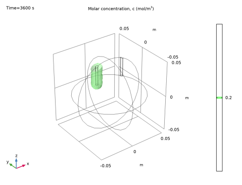
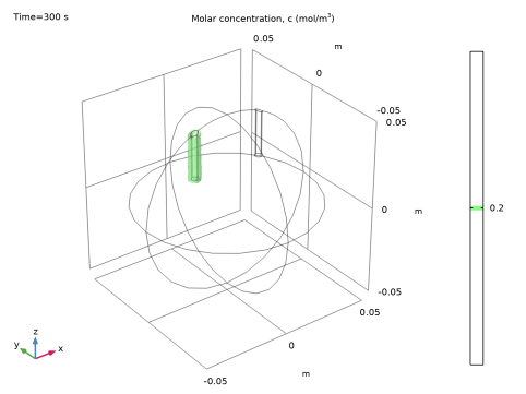
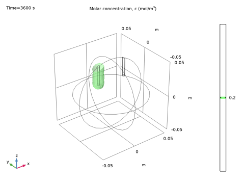
In the Settings window for Isosurface, click Replace Expression in the upper-right corner of the Expression section. From the menu, choose Component 1 (comp1) > Transport of Diluted Species > Species c > c - Molar concentration, c - mol/m³.
3
Locate the Levels section. From the Entry method list, choose Levels.
4
In the Levels text field, type 0.2.
5
Click the  Zoom Extents button in the Graphics toolbar.
6
In the Concentration Isosurface toolbar, click  Plot.
Animation 1
The following steps create an animation of the zinc ion isosurface during the simulated time:
1
In the Results toolbar, click  Animation and choose Player.
2
In the Settings window for Animation, locate the Scene section.
3
From the Subject list, choose Concentration Isosurface.
4
Locate the Animation Editing section. From the Time selection list, choose From list.
At t = 0 there is no concentration gradient in the orange. Therefore, clear the first time step.
5
In the Times (s) list, choose 60, 120, 180, 240, 300, 360, 420, 480, 540, 600, 660, 720, 780, 840, 900, 960, 1020, 1080, 1140, 1200, 1260, 1320, 1380, 1440, 1500, 1560, 1620, 1680, 1740, 1800, 1860, 1920, 1980, 2040, 2100, 2160, 2220, 2280, 2340, 2400, 2460, 2520, 2580, 2640, 2700, 2760, 2820, 2880, 2940, 3000, 3060, 3120, 3180, 3240, 3300, 3360, 3420, 3480, 3540, and 3600.
6
Click the  Zoom Extents button in the Graphics toolbar.
7
Click the  Play button in the Graphics toolbar.
Study 1
Step 1: Stationary
Note that if you want to experiment with the model by changing parameter values and simulate new polarization plots using the first (stationary) study, you have to disable the Transport of Diluted Species interface in that study as follows:
1
In the Model Builder window, under Study 1 click Step 1: Stationary.
2
In the Settings window for Stationary, locate the Physics and Variables Selection section.
3
In the Solve for column of the table, under Component 1 (comp1), clear the checkbox for Transport of Diluted Species (tds).