|
|
|
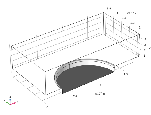


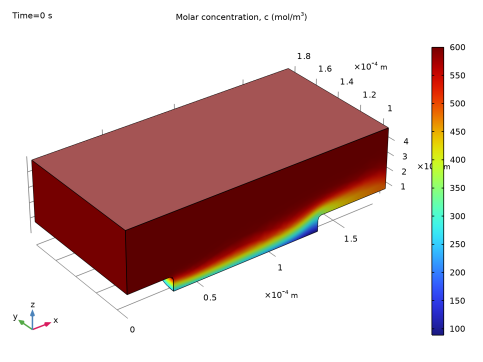
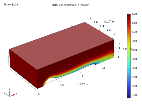
 the electrolyte cupric ion concentration (mol/m3), and
  , the reference cupric concentration in the bulk electrolyte (600 mol/m3).
|
1
|
|
2
|
In the Select Physics tree, select Electrochemistry > Electrodeposition, Deformed Geometry > Electrodeposition, Tertiary with Supporting Electrolyte.
|
|
3
|
Click Add.
|
|
4
|
|
5
|
In the Concentrations (mol/m³) table, enter the following settings:
|
|
6
|
|
7
|
Click Add.
|
|
8
|
Click
 Done. Done. |
|
1
|
|
2
|
|
3
|
Click
 Load from File. Load from File. |
|
4
|
Browse to the model’s Application Libraries folder and double-click the file microconnector_bump_parameters.txt.
|
|
1
|
In the Model Builder window, under Component 1 (comp1) right-click Definitions and choose Variables.
|
|
2
|
|
3
|
Click
 Load from File. Load from File. |
|
4
|
Browse to the model’s Application Libraries folder and double-click the file microconnector_bump_3d_variables.txt.
|
|
1
|
|
2
|
|
3
|
|
4
|
|
5
|
|
6
|
|
1
|
|
2
|
|
3
|
|
4
|
|
5
|
|
6
|
|
7
|
Click
 Build Selected. Build Selected. |
|
8
|
|
1
|
|
2
|
|
3
|
|
4
|
|
5
|
|
6
|
Click
 Build Selected. Build Selected. |
|
1
|
|
2
|
|
3
|
|
4
|
|
5
|
|
6
|
|
7
|
|
8
|
Click
 Build Selected. Build Selected. |
|
1
|
|
2
|
Select the object cyl2 only.
|
|
3
|
|
4
|
|
5
|
Select the object tor1 only.
|
|
6
|
Click
 Build Selected. Build Selected. |
|
1
|
|
2
|
Click in the Graphics window and then press Ctrl+A to select all objects.
|
|
3
|
|
4
|
Clear the Keep interior boundaries checkbox.
|
|
5
|
Click
 Build Selected. Build Selected. |
|
1
|
|
2
|
|
3
|
|
4
|
|
1
|
|
2
|
Select the object uni1 only.
|
|
3
|
|
4
|
|
5
|
Click
 Build Selected. Build Selected. |
|
1
|
|
2
|
|
3
|
|
4
|
|
5
|
Click
 Build Selected. Build Selected. |
|
6
|
|
1
|
|
2
|
|
3
|
|
5
|
|
1
|
|
2
|
|
3
|
|
5
|
|
1
|
|
2
|
|
3
|
|
5
|
|
1
|
|
2
|
|
3
|
|
5
|
|
1
|
|
2
|
|
3
|
|
5
|
|
1
|
|
2
|
|
3
|
|
4
|
|
5
|
|
6
|
Click OK.
|
|
7
|
|
1
|
|
2
|
|
3
|
|
5
|
|
1
|
In the Model Builder window, under Component 1 (comp1) > Tertiary Current Distribution, Nernst–Planck (tcd) click Electrolyte 1.
|
|
2
|
|
3
|
|
4
|
|
5
|
Locate the Solvent section. From the σl list, choose User defined. In the associated text field, type 1.
|
|
1
|
|
2
|
|
3
|
|
1
|
|
2
|
|
3
|
|
4
|
|
5
|
|
1
|
|
2
|
In the Settings window for Electrolyte Potential, type Electrolyte Potential - Bulk in the Label text field.
|
|
3
|
|
1
|
|
2
|
In the Settings window for Electrode Surface, click to expand the Dissolving–Depositing Species section.
|
|
3
|
Click
 Add. Add. |
|
4
|
Clear the Solve for surface concentration variables checkbox.
|
|
5
|
|
6
|
|
1
|
|
2
|
|
3
|
|
4
|
|
5
|
In the Stoichiometric coefficients for dissolving–depositing species: table, enter the following settings:
|
|
6
|
Click to expand the Reference Concentrations section. In the table, enter the following settings:
|
|
7
|
|
8
|
|
1
|
|
2
|
|
3
|
|
4
|
|
5
|
In the Settings window for Tertiary Current Distribution, Nernst–Planck, click to expand the Discretization section.
|
|
6
|
|
7
|
|
8
|
|
1
|
In the Model Builder window, under Component 1 (comp1) > Laminar Flow (spf) click Fluid Properties 1.
|
|
2
|
|
3
|
|
4
|
|
1
|
|
2
|
|
3
|
|
1
|
|
2
|
|
3
|
|
4
|
|
5
|
|
1
|
|
2
|
|
3
|
|
4
|
|
5
|
|
1
|
|
2
|
|
3
|
|
1
|
|
3
|
|
4
|
|
1
|
|
2
|
|
3
|
|
4
|
|
5
|
|
6
|
Locate the Element Size Parameters section.
|
|
7
|
|
1
|
|
2
|
|
3
|
|
4
|
|
5
|
|
1
|
|
2
|
|
3
|
|
4
|
Click to expand the Advanced Settings section. From the Interpolation method list, choose Transfinite in 3D.
|
|
1
|
|
2
|
|
3
|
|
4
|
|
5
|
Click
 Build Selected. Build Selected. |
|
1
|
|
2
|
|
1
|
|
2
|
|
3
|
|
4
|
|
1
|
|
3
|
|
4
|
|
5
|
|
6
|
|
7
|
Click
 Build All. Build All. |
|
8
|
|
1
|
|
2
|
Go to the Add Study window.
|
|
3
|
|
4
|
Click the Add Study button in the window toolbar.
|
|
5
|
|
1
|
|
2
|
Select the Modify model configuration for study step checkbox.
|
|
3
|
|
4
|
Click
 Disable in Solvers. Disable in Solvers. |
|
5
|
In the tree, select Component 1 (comp1) > Multiphysics > Nondeforming Boundary 1 (ndbdg1), Component 1 (comp1) > Multiphysics > Deforming Electrode Surface 1 (desdg1), and Component 1 (comp1) > Multiphysics > Nondeforming Boundary 2 (ndbdg2).
|
|
6
|
Click
 Disable in Solvers. Disable in Solvers. |
|
1
|
|
2
|
|
3
|
Select the Modify model configuration for study step checkbox.
|
|
4
|
|
5
|
Right-click and choose Disable in Solvers.
|
|
6
|
In the tree, select Component 1 (comp1) > Multiphysics > Nondeforming Boundary 1 (ndbdg1), Component 1 (comp1) > Multiphysics > Deforming Electrode Surface 1 (desdg1), and Component 1 (comp1) > Multiphysics > Nondeforming Boundary 2 (ndbdg2).
|
|
7
|
Right-click and choose Disable in Solvers.
|
|
1
|
|
2
|
|
3
|
|
1
|
|
2
|
|
3
|
In the Model Builder window, expand the Study 1 > Solver Configurations > Solution 1 (sol1) > Time-Dependent Solver 1 node, then click Segregated 1.
|
|
4
|
|
5
|
|
6
|
In the Model Builder window, expand the Study 1 > Solver Configurations > Solution 1 (sol1) > Time-Dependent Solver 1 > Segregated 1 node, then click Velocity u, Pressure p.
|
|
7
|
|
8
|
|
9
|
In the Model Builder window, under Study 1 > Solver Configurations > Solution 1 (sol1) > Time-Dependent Solver 1 > Segregated 1 click Merged Variables.
|
|
10
|
|
11
|
|
12
|
|
13
|
|
14
|
Clear the Generate default plots checkbox.
|
|
15
|
|
1
|
|
2
|
|
1
|
|
2
|
|
3
|
|
4
|
|
5
|
|
1
|
|
2
|
|
3
|
|
4
|
|
1
|
|
2
|
|
3
|
|
4
|
|
5
|
|
6
|
|
1
|
|
2
|
|
3
|
|
4
|
|
5
|
|
6
|
|
7
|
Click Define custom colors.
|
|
9
|
Click Add to custom colors.
|
|
10
|
|
11
|
|
12
|
|
1
|
|
1
|
|
2
|
|
3
|
|
4
|
|
5
|
|
6
|
|
7
|
|
8
|
|
1
|
|
2
|
|
3
|
Click
 Paste Selection. Paste Selection. |
|
4
|
|
5
|
Click OK.
|
|
1
|
|
2
|
|
3
|
|
4
|
|
1
|
|
2
|
|
3
|
Click
 Clear Selection. Clear Selection. |
|
4
|
Click
 Paste Selection. Paste Selection. |
|
5
|
|
6
|
Click OK.
|
|
1
|
|
2
|
|
3
|
|
4
|
|
5
|
|
6
|
|
1
|
|
2
|
|
3
|
Click
 Paste Selection. Paste Selection. |
|
4
|
|
5
|
Click OK.
|
|
1
|
|
2
|
|
3
|
|
4
|
|
5
|
|
6
|